SESAME
SESAME is an open-source Python tool designed to make spatial data analysis, visualization, and exploration accessible to all.
Whether you’re a researcher, student, or enthusiast, SESAME helps you unlock insights from geospatial data with just a few lines of code.
What can you do with the SESAME toolbox?
- Conveniently process and analyze both spatial datasets (e.g. GeoTIFFs) and tabular jurisdictional data (e.g. csv files by country) through a unified set of tools.
- Generate standardized netcdf files from a wide range of spatial input types (e.g. lines, points, polygons)
- Create publication-ready maps and plots.
- Explore spatial and temporal patterns among hundreds of variables in the Human-Earth Atlas.
Getting Started with the Human-Earth Atlas:
- Install SESAME*
- Download the Human-Earth Atlas (Figshare Link)
- Load your spatial data (e.g., land cover, population, climate)
- Use SESAME’s plotting tools to visualize and compare datasets
- Explore spatial and temporal patterns among hundreds of variables in the Human-Earth Atlas.
*Note: SESAME may take up to 2 minutes to load when used for the first time. This will not recur with further use.
Navigating the Atlas:
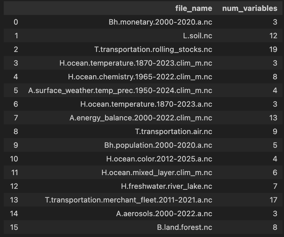
- List the netCDF files in the Human–Earth Atlas
import sesame as ssm
ssm.atlas(directory=atlas)
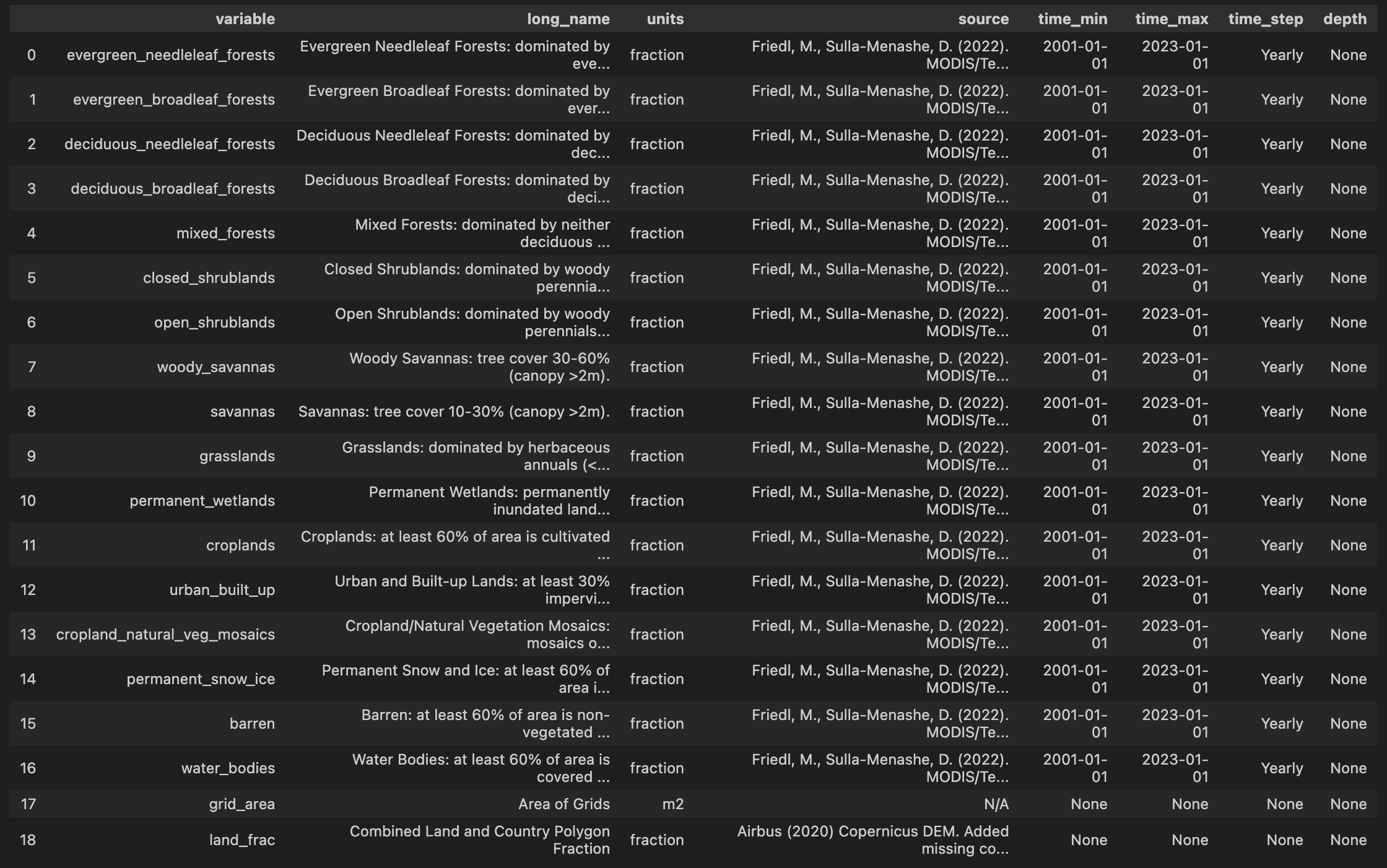
- View dataset metadata
ssm.list_variables("atlas/B.land.cover.2001-2023.a.nc")
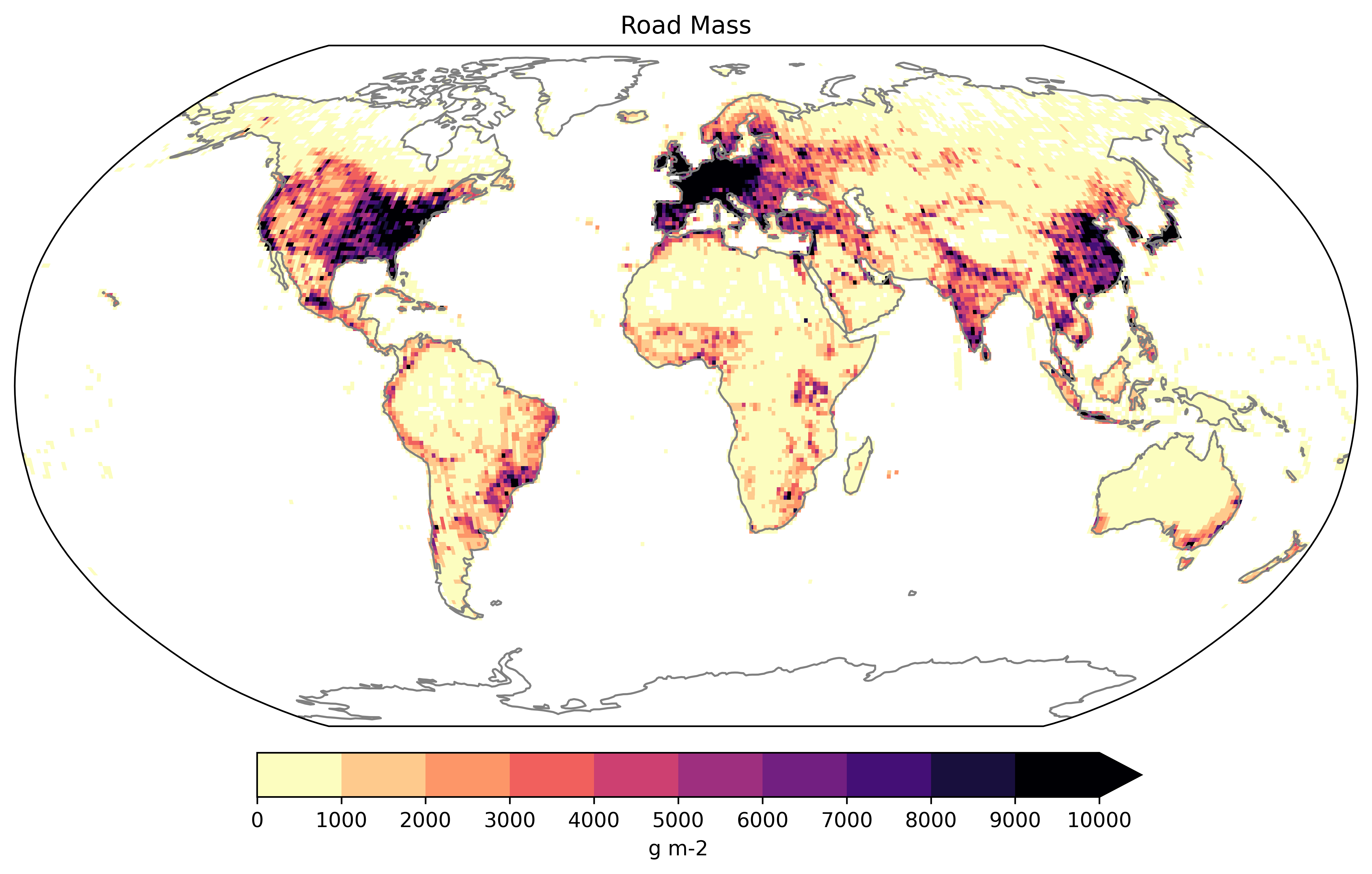
- Visualize data on the map
# Load data
netcdf_file = "atlas/T.transportation.roads.nc"
ssm.plot_map(dataset=netcdf_file,variable="roads_gross", color='magma_r', title='Gross Road Mass', label='g m-2', vmin=0, vmax=1e4, extend_max=True)
- Quick mathematical operation
# Load data
netcdf_file = "atlas/T.transportation.roads.nc"
# Perform the operation
ssm.divide_variables(dataset=netcdf_file, variable1="road_length", variable2="grid_area", new_variable_name="road_density")
Ready to get started? Dive into the function docs below or read The SESAME Human-Earth Atlas paper for inspiration!
1""" 2SESAME is an open-source Python tool designed to make spatial data analysis, visualization, and exploration accessible to all. 3Whether you’re a researcher, student, or enthusiast, SESAME helps you unlock insights from geospatial data with just a few lines of code. 4 5--- 6 7**What can you do with the SESAME toolbox?** 8 9- Conveniently process and analyze both spatial datasets (e.g. GeoTIFFs) and tabular jurisdictional data (e.g. csv files by country) through a unified set of tools. 10- Generate standardized netcdf files from a wide range of spatial input types (e.g. lines, points, polygons) 11- Create publication-ready maps and plots. 12- Explore spatial and temporal patterns among hundreds of variables in the Human-Earth Atlas. 13 14**Getting Started with the Human-Earth Atlas:** 15 161. Install SESAME* 172. Download the Human-Earth Atlas ([Figshare Link](https://doi.org/10.6084/m9.figshare.28432499)) 183. Load your spatial data (e.g., land cover, population, climate) 194. Use SESAME’s plotting tools to visualize and compare datasets 205. Explore spatial and temporal patterns among hundreds of variables in the Human-Earth Atlas. 21 22*Note: SESAME may take up to 2 minutes to load when used for the first time. This will not recur with further use. 23 24**Navigating the Atlas:** 251. List the netCDF files in the Human–Earth Atlas 26```python 27import sesame as ssm 28ssm.atlas(directory=atlas) 29``` 30<img src="../images/atlas.png" alt="Human-Earth Atlas" width="600"/> 31 322. View dataset metadata 33```python 34ssm.list_variables("atlas/B.land.cover.2001-2023.a.nc") 35``` 36<img src="../images/info.png" alt="NetCDF Info" width="600"/> 37 383. Visualize data on the map 39```python 40# Load data 41netcdf_file = "atlas/T.transportation.roads.nc" 42ssm.plot_map(dataset=netcdf_file,variable="roads_gross", color='magma_r', title='Gross Road Mass', label='g m-2', vmin=0, vmax=1e4, extend_max=True) 43``` 44<img src="../images/gross_road.png" alt="Gross Road Mass Map" width="600"/> 45 464. Quick mathematical operation 47```python 48# Load data 49netcdf_file = "atlas/T.transportation.roads.nc" 50# Perform the operation 51ssm.divide_variables(dataset=netcdf_file, variable1="road_length", variable2="grid_area", new_variable_name="road_density") 52``` 53 54Ready to get started? Dive into the function docs below or read [The SESAME Human-Earth Atlas](https://www.nature.com/articles/s41597-025-05087-5) paper for inspiration! 55 56--- 57""" 58 59import os 60import geopandas as gpd 61import pandas as pd 62import numpy as np 63import xarray as xr 64import json 65 66from . import create 67from . import utils 68from . import calculate 69from . import plot 70from . import get 71 72# import create 73# import utils 74# import calculate 75# import plot 76# import get 77 78 79def point_2_grid(point_data, variable_name='variable', long_name='variable', units="value/grid-cell", source=None, time=None, resolution=1, agg_column=None, agg_function="sum", attr_field=None, output_directory=None, output_filename=None, normalize_by_area=False, zero_is_value=False, verbose=False): 80 81 """ 82 Converts point data from a shapefile or GeoDataFrame into a gridded netCDF dataset. 83 84 Parameters 85 ---------- 86 - point_data : GeoDataFrame or str. Input point data to be gridded. Can be either a GeoDataFrame or a path to a point shapefile (.shp). 87 - variable_name : str, optional. Name of the variable to include in the netCDF attributes metadata. Defaults to: 88 - The unique entries in the `attr_field` column if specified. 89 - The input filename without extension if `attr_field` and `variable_name` are not specified. 90 - long_name : str, optional. A descriptive name for the variable, added to the netCDF metadata. Behaves the same as `variable_name` if 91 `attr_field` is specified. Defaults to the input filename without extension if unspecified. 92 - units : str, optional. Units of the data variable to include in the netCDF metadata. Default is "value/grid-cell". 93 - source : str, optional. String describing the original source of the input data. This will be added to the netCDF metadata. 94 - time : str, optional. Time dimension for the output netCDF. If specified, the output will include a time dimension with the 95 value provided. Default is None (spatial, 2D netCDF output). 96 - resolution : float, optional. Desired resolution for the grid cells in the output dataset. Default is 1 degree. 97 - agg_column : str, optional. Column name in the shapefile or GeoDataFrame specifying the values to aggregate in each grid cell. 98 Defaults to counting the number of points per grid cell. 99 - agg_function : str, optional. Aggregation method for combining values in each grid cell. Options include: 100 - 'sum' (default): Sums all point values. 101 - 'max': Takes the maximum value. 102 - 'min': Takes the minimum value. 103 - 'std': Computes the standard deviation. 104 - attr_field : str, optional. Column name in the shapefile or GeoDataFrame specifying the variable names for multiple data types. 105 - output_directory : str, optional. Directory where the output NetCDF file will be saved. If None, but output_filename is True, the file will be saved in the current working directory. 106 - output_filename : str, optional. Name of the output NetCDF file (without the `.nc` extension). If not provided: 107 - Uses the input shapefile name if a shapefile path is given. 108 - Saves as `"gridded_points.nc"` if a GeoDataFrame is provided as input. 109 - normalize_by_area : bool, optional. If True, normalizes the grid values by area (e.g., converts to value per square meter). Default is False. 110 - zero_is_value : bool, optional. If True, treats zero values as valid data rather than as no-data. Default is False. 111 - verbose : bool, optional. If True, prints information about the process, such as global sum of values before and after gridding. Default is False. 112 113 Returns 114 ------- 115 - xarray.Dataset. Transformed dataset with gridded data derived from the input point data. 116 117 Notes 118 ----- 119 - The function supports input in the form of a shapefile or GeoDataFrame containing point data. 120 - If points lie exactly on a grid boundary, they are shifted by 0.0001 degrees in both latitude and longitude to ensure assignment to a grid cell. 121 - The function creates a netCDF file, where data variables are aggregated based on the `agg_column` and `agg_function`. 122 123 Example 124 ------- 125 >>> point_2_grid(point_data=shapefile_path, 126 ... variable_name="airplanes", 127 ... long_name="Airplanes Count", 128 ... units="airport/grid-cell", 129 ... source="CIA", 130 ... resolution=1, 131 ... verbose=True 132 ... ) 133 134 """ 135 136 # Determine if input is a path (string or Path) or a GeoDataFrame 137 if isinstance(point_data, (str, bytes, os.PathLike)): 138 if verbose: 139 print("Reading shapefile from path...") 140 points_gdf = gpd.read_file(point_data) 141 elif isinstance(point_data, gpd.GeoDataFrame): 142 points_gdf = point_data 143 else: 144 raise TypeError("Input must be a GeoDataFrame or a shapefile path (string or Path).") 145 146 # create gridded polygon 147 polygons_gdf = create.create_gridded_polygon(resolution=resolution, out_polygon_path=None, grid_area=False) 148 149 if attr_field is not None: 150 unique_rows = points_gdf[attr_field].unique().tolist() 151 dataset_list = [] 152 153 for filter_var in unique_rows: 154 # Filter the GeoDataFrame 155 filtered_gdf = points_gdf[points_gdf[attr_field] == filter_var].copy() 156 joined_gdf = utils.point_spatial_join(polygons_gdf, filtered_gdf, agg_column=agg_column, agg_function=agg_function) 157 158 # Determine agg_column, long_name, and units for the current iteration 159 current_agg_column = agg_column or "count" 160 current_long_name = utils.reverse_replace_special_characters(filter_var) 161 current_units = utils.determine_units_point(units, normalize_by_area) 162 163 # Convert joined GeoDataFrame to xarray dataset 164 ds_var = utils.gridded_poly_2_xarray( 165 polygon_gdf=joined_gdf, 166 grid_value=current_agg_column, 167 long_name=current_long_name, 168 units=current_units, 169 source=source, 170 time=time, 171 resolution=resolution, 172 variable_name=filter_var, 173 normalize_by_area=normalize_by_area, 174 zero_is_value=zero_is_value 175 ) 176 177 # Print or process verbose information 178 if verbose: 179 global_summary_stats = utils.dataframe_stats_point(dataframe=filtered_gdf, agg_column=current_agg_column, agg_function=agg_function) 180 print(f"Global stats of {filter_var} before gridding : {global_summary_stats:.2f}") 181 var_name = utils.replace_special_characters(filter_var) 182 global_gridded_stats = utils.xarray_dataset_stats(dataset=ds_var, variable_name=var_name, normalize_by_area=normalize_by_area, resolution=resolution) 183 print(f"Global stats of {filter_var} after gridding: {global_gridded_stats:.2f}") 184 185 print("\n") 186 dataset_list.append(ds_var) 187 188 # Merge all datasets from different filtered GeoDataFrames 189 ds = xr.merge(dataset_list) 190 191 else: 192 joined_gdf = utils.point_spatial_join(polygons_gdf, points_gdf, agg_column=agg_column, agg_function=agg_function) 193 194 # Determine agg_column, long_name, and units 195 agg_column = agg_column or "count" 196 long_name = utils.determine_long_name_point(agg_column, variable_name, long_name, agg_function) 197 units = utils.determine_units_point(units, normalize_by_area) 198 199 ds = utils.gridded_poly_2_xarray( 200 polygon_gdf=joined_gdf, 201 grid_value=agg_column, 202 long_name=long_name, 203 units=units, 204 source=source, 205 time=time, 206 resolution=resolution, 207 variable_name=variable_name, 208 normalize_by_area=normalize_by_area, 209 zero_is_value=zero_is_value 210 ) 211 212 if verbose: 213 global_summary_stats = utils.dataframe_stats_point(dataframe=points_gdf, agg_column=agg_column, agg_function=agg_function) 214 print(f"Global stats before gridding : {global_summary_stats:.2f}") 215 global_gridded_stats = utils.xarray_dataset_stats(dataset=ds, variable_name=variable_name, normalize_by_area=normalize_by_area, resolution=resolution) 216 print(f"Global stats after gridding: {global_gridded_stats:.2f}") 217 218 if output_directory or output_filename: 219 # Set output directory 220 output_directory = (output_directory or os.getcwd()).rstrip(os.sep) + os.sep 221 # Set base filename 222 base_filename = os.path.splitext(os.path.basename(point_data))[0] if isinstance(point_data, (str, bytes, os.PathLike)) else "gridded_points" 223 # Set output filename 224 output_filename = output_filename or base_filename 225 # save the xarray dataset 226 utils.save_to_nc(ds, output_directory=output_directory, output_filename=output_filename, base_filename=base_filename) 227 return ds 228 229def line_2_grid(line_data, variable_name='variable', long_name='variable', units="meter/grid-cell", source=None, time=None, resolution=1, agg_column=None, agg_function="sum", attr_field=None, output_directory=None, output_filename=None, normalize_by_area=False, zero_is_value=False, verbose=False): 230 231 """ 232 Converts line data from a shapefile or GeoDataFrame into a gridded netCDF dataset. 233 234 Parameters 235 ---------- 236 - line_data : GeoDataFrame or str. Input lines data to be gridded. Can be either a GeoDataFrame or a path to a line/polyline shapefile (.shp). 237 - variable_name : str, optional. Name of the variable to include in the netCDF attributes metadata. Defaults to: 238 - The unique entries in the `attr_field` column if specified. 239 - The input filename without extension if `attr_field` and `variable_name` are not specified. 240 - long_name : str, optional. A descriptive name for the variable, added to the netCDF metadata. Behaves the same as `variable_name` if 241 `attr_field` is specified. Defaults to the input filename without extension if unspecified. 242 - units : str, optional. Units of the data variable to include in the netCDF metadata. Default is "meter/grid-cell". 243 - source : str, optional. String describing the original source of the input data. This will be added to the netCDF metadata. 244 - time : str, optional. Time dimension for the output netCDF. If specified, the output will include a time dimension with the 245 value provided. Default is None (spatial, 2D netCDF output). 246 - resolution : float, optional. Desired resolution for the grid cells in the output dataset. Default is 1 degree. 247 - agg_column : str, optional. Column name in the shapefile or GeoDataFrame specifying the values to aggregate in each grid cell. 248 Defaults to summing the lengths of intersected lines per grid cell. 249 - agg_function : str, optional. Aggregation method for combining values in each grid cell. Options include: 250 - 'sum' (default): Sums all line values. 251 - 'max': Takes the maximum value. 252 - 'min': Takes the minimum value. 253 - 'std': Computes the standard deviation. 254 - attr_field : str, optional. Column name in the shapefile or GeoDataFrame specifying the variable names for multiple data types. 255 - output_directory : str, optional. Directory where the output NetCDF file will be saved. If None, but output_filename is True, the file will be saved in the current working directory. 256 - output_filename : str, optional. Name of the output NetCDF file (without the `.nc` extension). If not provided: 257 - Uses the input shapefile name if a shapefile path is given. 258 - Saves as `"gridded_lines.nc"` if a GeoDataFrame is provided as input. 259 - normalize_by_area : bool, optional. If True, normalizes the variable in each grid cell by the area of the grid cell (e.g., converts to value per square meter). Default is False. 260 - zero_is_value : bool, optional. If True, treats zero values as valid data rather than as no-data. Default is False. 261 If True, treats zero values as valid data rather than as no-data. Default is False. 262 - verbose : bool, optional. If True, prints information about the process, such as global sum of values before and after gridding. Default is False. 263 264 Returns 265 ------- 266 - xarray.Dataset. Transformed dataset with gridded data derived from the input line data. 267 268 Notes 269 ----- 270 - The function supports input in the form of a shapefile or GeoDataFrame containing line data. 271 - Line lengths are calculated and aggregated based on the specified `agg_column` and `agg_function`. 272 - If lines intersect a grid boundary, their contributions are divided proportionally among the intersected grid cells. 273 - The function creates a netCDF file, where data variables are aggregated and stored with metadata. 274 275 Example 276 ------- 277 >>> line_2_grid(line_data=shapefile_path, 278 ... variable_name="roads", 279 ... long_name="Roads Length", 280 ... units="meter/grid-cell", 281 ... source="OpenStreetMap", 282 ... resolution=1, 283 ... agg_function="sum", 284 ... verbose=True) 285 ... ) 286 287 """ 288 289 # Determine if input is a path (string or Path) or a GeoDataFrame 290 if isinstance(line_data, (str, bytes, os.PathLike)): 291 if verbose: 292 print("Reading shapefile from path...") 293 lines_gdf = gpd.read_file(line_data) 294 elif isinstance(line_data, gpd.GeoDataFrame): 295 lines_gdf = line_data 296 else: 297 raise TypeError("Input must be a GeoDataFrame or a shapefile path (string or Path).") 298 299 # create gridded polygon 300 polygons_gdf = create.create_gridded_polygon(resolution=resolution, out_polygon_path=None, grid_area=False) 301 302 if attr_field is not None: 303 unique_rows = lines_gdf[attr_field].unique().tolist() 304 dataset_list = [] 305 306 for filter_var in unique_rows: 307 # Filter the GeoDataFrame 308 filtered_gdf = lines_gdf[lines_gdf[attr_field] == filter_var].copy() 309 joined_gdf = utils.line_intersect(polygons_gdf, filtered_gdf, agg_column=agg_column, agg_function=agg_function) 310 311 # Determine agg_column, long_name, and units for the current iteration 312 current_agg_column = agg_column or f"length_{agg_function.lower()}" 313 current_long_name = utils.reverse_replace_special_characters(filter_var) 314 current_units = utils.determine_units_line(units, normalize_by_area) 315 316 # Convert joined GeoDataFrame to xarray dataset 317 ds_var = utils.gridded_poly_2_xarray( 318 polygon_gdf=joined_gdf, 319 grid_value=current_agg_column, 320 long_name=current_long_name, 321 units=current_units, 322 source=source, 323 time=time, 324 resolution=resolution, 325 variable_name=filter_var, 326 normalize_by_area=normalize_by_area, 327 zero_is_value=zero_is_value 328 ) 329 330 # Print or process verbose information 331 if verbose: 332 global_summary_stats = utils.dataframe_stats_line(dataframe=filtered_gdf, agg_column=agg_column, agg_function=agg_function) 333 print(f"Global stats of {filter_var} before gridding : {global_summary_stats:.2f} km.") 334 var_name = utils.replace_special_characters(filter_var) 335 global_gridded_stats = utils.xarray_dataset_stats(dataset=ds_var, variable_name=var_name, normalize_by_area=normalize_by_area, resolution=resolution) * 1e-3 336 print(f"Global stats of {filter_var} after gridding: {global_gridded_stats:.2f} km.") 337 338 print("\n") 339 dataset_list.append(ds_var) 340 341 # Merge all datasets from different filtered GeoDataFrames 342 ds = xr.merge(dataset_list) 343 344 else: 345 joined_gdf = utils.line_intersect(polygons_gdf, lines_gdf, agg_column=agg_column, agg_function=agg_function) 346 347 # Determine agg_column, long_name, and units 348 agg_column = agg_column or "length_m" 349 long_name = utils.determine_long_name_line(long_name, agg_column, variable_name) 350 units = utils.determine_units_line(units, normalize_by_area) 351 ds = utils.gridded_poly_2_xarray( 352 polygon_gdf=joined_gdf, 353 grid_value=agg_column, 354 long_name=long_name, 355 units=units, 356 source=source, 357 time=time, 358 resolution=resolution, 359 variable_name=variable_name, 360 normalize_by_area=normalize_by_area, 361 zero_is_value=zero_is_value 362 ) 363 364 if verbose: 365 if agg_column == "length_m": 366 global_summary_stats = utils.dataframe_stats_line(dataframe=lines_gdf, agg_column=agg_column, agg_function=agg_function) 367 print(f"Global stats before gridding : {global_summary_stats:.2f} km.") 368 global_gridded_stats = utils.xarray_dataset_stats(dataset=ds, variable_name=variable_name, agg_column=agg_column, normalize_by_area=normalize_by_area, resolution=resolution) * 1e-3 369 print(f"Global stats after gridding: {global_gridded_stats:.2f} km.") 370 else: 371 global_summary_stats = utils.dataframe_stats_line(dataframe=lines_gdf, agg_column=agg_column, agg_function=agg_function) 372 print(f"Global stats before gridding : {global_summary_stats:.2f}.") 373 global_gridded_stats = utils.xarray_dataset_stats(dataset=ds, variable_name=variable_name, agg_column=agg_column, normalize_by_area=normalize_by_area, resolution=resolution) 374 print(f"Global stats after gridding: {global_gridded_stats:.2f}.") 375 376 if output_directory or output_filename: 377 # Set output directory 378 output_directory = (output_directory or os.getcwd()).rstrip(os.sep) + os.sep 379 # Set base filename 380 base_filename = os.path.splitext(os.path.basename(line_data))[0] if isinstance(line_data, (str, bytes, os.PathLike)) else "gridded_lines" 381 # Set output filename 382 output_filename = output_filename or base_filename 383 # save the xarray dataset 384 utils.save_to_nc(ds, output_directory=output_directory, output_filename=output_filename, base_filename=base_filename) 385 return ds 386 387def poly_2_grid(polygon_data, variable_name='variable', long_name='variable', units="m2/grid-cell", source=None, time=None, resolution=1, attr_field=None, fraction=False, agg_function="sum", output_directory=None, output_filename=None, normalize_by_area=False, zero_is_value=False, verbose=False): 388 389 """ 390 Converts polygon data from a shapefile or GeoDataFrame into a gridded netCDF dataset. 391 392 Parameters 393 ---------- 394 - polygon_data : GeoDataFrame or str. Input polygons data to be gridded. Can be either a GeoDataFrame or a path to a polygons shapefile (.shp). 395 - variable_name : str, optional. Name of the variable to include in the netCDF attributes metadata. Defaults to: 396 - The unique entries in the `attr_field` column if specified. 397 - The input filename without extension if `attr_field` and `variable_name` are not specified. 398 - long_name : str, optional. A descriptive name for the variable, added to the netCDF metadata. Behaves the same as `variable_name` if 399 `attr_field` is specified. Defaults to the input filename without extension if unspecified. 400 - units : str, optional. Units of the data variable to include in the netCDF metadata. Default is "m2/grid-cell". 401 - source : str, optional. String describing the original source of the input data. This will be added to the netCDF metadata. 402 - time : str, optional. Time dimension for the output netCDF. If specified, the output will include a time dimension with the 403 value provided. Default is None (spatial, 2D netCDF output). 404 - resolution : float, optional. Desired resolution for the grid cells in the output dataset. Default is 1 degree. 405 - attr_field : str, optional. Column name in the shapefile or GeoDataFrame specifying the variable names for multiple data types. 406 - fraction : bool, optional. If True, calculates the fraction of each polygon within each grid cell. The output values will range from 0 to 1. Default is False. 407 - agg_function : str, optional. Aggregation method for combining values in each grid cell. Default is 'sum'. Options include: 408 - 'sum': Sum of values. 409 - 'max': Maximum value. 410 - 'min': Minimum value. 411 - 'std': Standard deviation. 412 - output_directory : str, optional. Directory where the output NetCDF file will be saved. If None, but output_filename is True, the file will be saved in the current working directory. 413 - output_filename : str, optional. Name of the output NetCDF file (without the `.nc` extension). If not provided: 414 - Uses the input shapefile name if a shapefile path is given. 415 - Saves as `"gridded_polygons.nc"` if a GeoDataFrame is provided as input. 416 - normalize_by_area : bool, optional. If True, normalizes the grid values by area (e.g., converts to value per square meter). Default is False. 417 - zero_is_value : bool, optional. If True, treats zero values as valid data rather than as no-data. Default is False. 418 - verbose : bool, optional. If True, prints information about the process, such as global sum of values before and after gridding. Default is False. 419 420 Returns 421 ------- 422 - xarray.Dataset. Transformed dataset with gridded data derived from the input polygon data. 423 424 Notes 425 ----- 426 - The function supports input in the form of a shapefile or GeoDataFrame containing polygon data. 427 - Polygon areas are calculated and aggregated based on the specified `attr_field` and `agg_function`. 428 - If the `fraction` parameter is True, the fraction of each polygon in each grid cell will be computed, with values ranging from 0 to 1. 429 - The function creates a netCDF file, where data variables are aggregated and stored with metadata. 430 431 Example 432 ------- 433 >>> poly_2_grid(polygon_data=shapefile_path, 434 ... units="fraction", 435 ... source="The new global lithological map database GLiM", 436 ... resolution=1, 437 ... attr_field="Short_Name", 438 ... fraction="yes", 439 ... verbose=True 440 ... ) 441 442 """ 443 444 # Determine if input is a path (string or Path) or a GeoDataFrame 445 if isinstance(polygon_data, (str, bytes, os.PathLike)): 446 if verbose: 447 print("Reading shapefile from path...") 448 poly_gdf = gpd.read_file(polygon_data) 449 elif isinstance(polygon_data, gpd.GeoDataFrame): 450 poly_gdf = polygon_data 451 else: 452 raise TypeError("Input must be a GeoDataFrame or a shapefile path (string or Path).") 453 454 # create gridded polygon 455 polygons_gdf = create.create_gridded_polygon(resolution=resolution, out_polygon_path=None, grid_area=False) 456 457 if attr_field is not None: 458 unique_rows = poly_gdf[attr_field].unique().tolist() 459 dataset_list = [] 460 461 for filter_var in unique_rows: 462 463 # Filter the GeoDataFrame 464 filtered_gdf = poly_gdf[poly_gdf[attr_field] == filter_var].copy() 465 # Reset the index to ensure sequential indexing 466 filtered_gdf.reset_index(drop=True, inplace=True) 467 468 # Determine agg_column, long_name, and units for the current iteration 469 grid_value = "frac" if fraction else "in_area" 470 current_long_name = utils.reverse_replace_special_characters(filter_var) 471 current_units = utils.determine_units_poly(units, normalize_by_area, fraction) 472 473 # Convert GeoDataFrame to xarray dataset 474 ds_var = utils.poly_intersect(poly_gdf=filtered_gdf, 475 polygons_gdf=polygons_gdf, 476 variable_name=filter_var, 477 long_name=current_long_name, 478 units=current_units, 479 source=source, 480 time=time, 481 resolution=resolution, 482 agg_function=agg_function, 483 fraction=fraction, 484 normalize_by_area=normalize_by_area, 485 zero_is_value=zero_is_value) 486 487 # Print or process verbose information 488 if verbose: 489 global_summary_stats = utils.dataframe_stats_poly(dataframe=filtered_gdf, agg_function=agg_function) 490 print(f"Global stats of {filter_var} before gridding : {global_summary_stats:.2f} km2.") 491 filter_var = utils.replace_special_characters(filter_var) 492 global_gridded_stats = utils.xarray_dataset_stats(dataset=ds_var, variable_name=filter_var, agg_column=grid_value, 493 normalize_by_area=True, resolution=resolution) * 1e-6 494 print(f"Global stats of {filter_var} after gridding: {global_gridded_stats:.2f} km2.") 495 496 print("\n") 497 dataset_list.append(ds_var) 498 499 # Merge all datasets from different filtered GeoDataFrames 500 ds = xr.merge(dataset_list) 501 502 else: 503 504 # Determine agg_column, long_name, and units 505 grid_value = "frac" if fraction else "in_area" 506 long_name = utils.determine_long_name_poly(variable_name, long_name, agg_function) 507 units = utils.determine_units_poly(units, normalize_by_area, fraction) 508 509 # Convert GeoDataFrame to xarray dataset 510 ds = utils.poly_intersect(poly_gdf=poly_gdf, 511 polygons_gdf=polygons_gdf, 512 variable_name=variable_name, 513 long_name=long_name, 514 units=units, 515 source=source, 516 time=time, 517 resolution=resolution, 518 agg_function=agg_function, 519 fraction=fraction, 520 normalize_by_area=normalize_by_area, 521 zero_is_value=zero_is_value) 522 523 if verbose: 524 global_summary_stats = utils.dataframe_stats_poly(dataframe=poly_gdf, agg_function=agg_function) 525 print(f"Global stats before gridding : {global_summary_stats:.2f} km2.") 526 variable_name = utils.replace_special_characters(variable_name) 527 if fraction: 528 normalize_by_area = True 529 global_gridded_stats = utils.xarray_dataset_stats(dataset=ds, variable_name=variable_name, agg_column=grid_value, 530 normalize_by_area=normalize_by_area, resolution=resolution) * 1e-6 531 print(f"Global stats after gridding: {global_gridded_stats:.2f} km2.") 532 533 if output_directory or output_filename: 534 # Set output directory 535 output_directory = (output_directory or os.getcwd()).rstrip(os.sep) + os.sep 536 # Set base filename 537 base_filename = os.path.splitext(os.path.basename(polygon_data))[0] if isinstance(polygon_data, (str, bytes, os.PathLike)) else "gridded_polygons" 538 # Set output filename 539 output_filename = output_filename or base_filename 540 # save the xarray dataset 541 utils.save_to_nc(ds, output_directory=output_directory, output_filename=output_filename, base_filename=base_filename) 542 return ds 543 544def grid_2_grid(raster_data, agg_function, variable_name, long_name, units="value/grid-cell", source=None, time=None, resolution=1, netcdf_variable=None, output_directory=None, output_filename=None, padding="symmetric", zero_is_value=False, normalize_by_area=False, verbose=False): 545 546 """ 547 Converts raster data (TIFF or netCDF) into a re-gridded xarray dataset. 548 549 Parameters 550 ---------- 551 - raster_data : str. Path to the input raster data file. This can be a string path to a TIFF (.tif) file, a string path to a NetCDF (.nc or .nc4) file or An already loaded xarray.Dataset object. 552 - If `raster_data` is a NetCDF file or an xarray.Dataset, the `netcdf_variable` parameter must also be provided to specify which variable to extract. 553 - agg_function : str. Aggregation method to apply when re-gridding. Supported values are 'SUM', 'MEAN', or 'MAX'. 554 - variable_name : str. Name of the variable to include in the output dataset. 555 - long_name : str. Descriptive name for the variable. 556 - units : str, optional. Units for the variable. Default is "value/grid-cell". 557 - source : str, optional. Source information for the dataset. Default is None. 558 - time : str or None, optional. Time stamp or identifier for the data. Default is None. 559 - resolution : int or float, optional. Desired resolution of the grid cells in degree in the output dataset. Default is 1. 560 - netcdf_variable : str, optional. Name of the variable to extract from the netCDF file, if applicable. Required for netCDF inputs. 561 - output_directory : str, optional. Directory where the output NetCDF file will be saved. If None, but output_filename is True, the file will be saved in the current working directory. 562 - output_filename : str, optional. Name of the output NetCDF file (without the `.nc` extension). If not provided: 563 - Uses `variable_name` if it is specified. 564 - Defaults to `regridded.nc` if none of the above are provided. 565 - padding : str, optional. Padding strategy ('symmetric' or 'end'). 566 - zero_is_value : bool, optional. Whether to treat zero values as valid data rather than as no-data. Default is False. 567 - normalize_by_area : bool, optional. Whether to normalize grid values by area (e.g., convert to value per square meter). Default is False. 568 - verbose : bool, optional. If True, prints the global sum of values before and after re-gridding. Default is False. 569 570 Returns 571 ------- 572 - xarray.Dataset. Re-gridded xarray dataset containing the processed raster data. 573 574 Notes 575 ----- 576 This function supports raster data in TIFF or netCDF format and performs re-gridding based on 577 the specified `agg_function`. The output dataset will include metadata such as the variable name, 578 long name, units, and optional source and time information. 579 580 Example 581 ------- 582 >>> grid_2_grid(raster_path=pop_path, 583 ... agg_function="sum", 584 ... variable_name="population_count", 585 ... long_name="Total Population", 586 ... units="people per grid", 587 ... source="WorldPop", 588 ... resolution=1, 589 ... time="2020-01-01", 590 ... verbose="yes" 591 ... ) 592 """ 593 594 # Determine the file extension 595 if isinstance(raster_data, (str, bytes, os.PathLike)): 596 file_extension = os.path.splitext(raster_data)[1].lower() 597 elif isinstance(raster_data, xr.Dataset): 598 file_extension = ".nc" 599 600 if file_extension == ".tif": 601 if verbose: 602 print("Reading the tif file.") 603 # Convert TIFF data to a re-gridded dataset 604 ds = utils.tif_2_ds(input_raster=raster_data, agg_function=agg_function, variable_name=variable_name, 605 long_name=long_name, units=units, source=source, resolution=resolution, time=time, padding=padding, 606 zero_is_value=zero_is_value, normalize_by_area=normalize_by_area, verbose=verbose) 607 608 elif file_extension == ".nc" or file_extension == ".nc4": 609 if verbose: 610 print("Reading the nc file.") 611 # Convert netCDF to TIFF 612 netcdf_tif_path, temp_path = utils.netcdf_2_tif(raster_data=raster_data, netcdf_variable=netcdf_variable, time=time) 613 # Convert netCDF data to a re-gridded dataset 614 ds = utils.tif_2_ds(input_raster=netcdf_tif_path, agg_function=agg_function, variable_name=variable_name, 615 long_name=long_name, units=units, source=source, resolution=resolution, time=time, padding=padding, 616 zero_is_value=zero_is_value, normalize_by_area=normalize_by_area, verbose=verbose) 617 # delete temp folder 618 utils.delete_temporary_folder(temp_path) 619 else: 620 # Print an error message for unrecognized file types 621 print("Error: File type is not recognized. File type should be either TIFF or netCDF file.") 622 623 if output_directory or output_filename: 624 # Set output directory 625 output_directory = (output_directory or os.getcwd()).rstrip(os.sep) + os.sep 626 # Set base filename 627 base_filename = variable_name or "regridded" 628 # Set output filename 629 output_filename = output_filename or base_filename 630 # save the xarray dataset 631 utils.save_to_nc(ds, output_directory=output_directory, output_filename=output_filename, base_filename=base_filename) 632 633 if verbose: 634 print("Re-gridding completed!") 635 return ds 636 637def table_2_grid(surrogate_data, surrogate_variable, tabular_data, tabular_column, variable_name=None, long_name=None, units="value/grid-cell", source=None, time=None, output_directory=None, output_filename=None, zero_is_value=False, normalize_by_area=False, eez=False, verbose=False): 638 """ 639 Convert tabular data to a gridded dataset by spatially distributing values based on a NetCDF variable and a tabular column. 640 641 Parameters: 642 ----------- 643 - surrogate_data : xarray.Dataset or str. xarray dataset or a path to a NetCDF file. If a file path is provided, it will be automatically loaded 644 into an xarray.Dataset. The dataset must include the variable specified in `surrogate_variable`. 645 - surrogate_variable : str. Variable name in the NetCDF or xarray dataset used for spatial distribution. 646 - tabular_data : pandas.DataFrame or str. Tabular dataset as a pandas DataFrame or a path to a CSV file. If a file path is provided, it will be 647 automatically loaded into a DataFrame. The data must include a column named "ISO3" representing country codes. 648 If not present, use the `add_iso3_column` utility function to convert country names to ISO3 codes. 649 - tabular_column : str. Column name in the tabular dataset with values to be spatially distributed. 650 - variable_name : str, optional. Name of the variable. Default is None. 651 - long_name : str, optional. A long name for the variable. Default is None. 652 - units : str, optional. Units of the variable. Default is 'value/grid'. 653 - source : str, optional. Source information, if available. Default is None. 654 - time : str, optional. Time information for the dataset. 655 - output_directory : str, optional. Directory where the output NetCDF file will be saved. If None, but output_filename is True, the file will be saved in the current working directory. 656 - output_filename : str, optional. Name of the output NetCDF file (without the `.nc` extension). If not provided: 657 - Uses `variable_name` if it is specified. 658 - Falls back to `long_name` or `tabular_column` if `variable_name` is not given. 659 - Defaults to `gridded_table.nc` if none of the above are provided. 660 - zero_is_value: bool, optional. If the value is True, then the function will treat zero as an existent value and 0 values will be considered while calculating mean and STD. 661 - normalize_by_area : bool, optional. Whether to normalize grid values by area (e.g., convert to value per square meter). Default is False. 662 - eez : bool, optional. If set to True, the function converts the jurisdictional Exclusive Economic Zone (EEZ) values to a spatial grid. 663 - verbose: bool, optional. If True, the global gridded sum of before and after re-gridding operation will be printed. If any jurisdiction where surrogate variable is missing and tabular data is evenly distributed over the jurisdiction, the ISO3 codes of evenly distributed countries will also be printed. 664 665 Returns: 666 -------- 667 - xarray.Dataset. Resulting gridded dataset after spatial distribution of tabular values. 668 669 Example 670 ------- 671 >>> table_2_grid(surrogate_data=netcdf_file_path, 672 ... surrogate_variable="railway_length", 673 ... tabular_data=csv_file_path, 674 ... tabular_column="steel", 675 ... variable_name="railtract_steel", 676 ... long_name="'Railtrack Steel Mass'", 677 ... units="g m-2", 678 ... source="Matitia (2022)", 679 ... normalize_by_area="yes", 680 ... verbose="yes" 681 ... ) 682 """ 683 684 # Load netcdf_file (either path or xarray.Dataset) 685 if isinstance(surrogate_data, (str, bytes, os.PathLike)): 686 input_ds = xr.open_dataset(surrogate_data) 687 elif isinstance(surrogate_data, xr.Dataset): 688 input_ds = surrogate_data 689 else: 690 raise TypeError("`netcdf_file` must be an xarray.Dataset or a path to a NetCDF file.") 691 692 # Load tabular_data (either path or pandas.DataFrame) 693 if isinstance(tabular_data, (str, bytes, os.PathLike)): 694 input_df = pd.read_csv(tabular_data) 695 elif isinstance(tabular_data, pd.DataFrame): 696 input_df = tabular_data 697 else: 698 raise TypeError("`tabular_data` must be a pandas.DataFrame or a path to a CSV file.") 699 700 if variable_name is None: 701 variable_name = long_name if long_name is not None else tabular_column 702 703 if long_name is None: 704 long_name = variable_name if variable_name is not None else tabular_column 705 706 # check the netcdf resolution 707 resolution = abs(float(input_ds['lat'].diff('lat').values[0])) 708 resolution_str = str(resolution) 709 710 if time: 711 # check and convert ISO3 based on occupation or previous control, given a specific year 712 input_df = utils.convert_iso3_by_year(df=input_df, year=time) 713 714 base_directory = os.path.dirname(os.path.abspath(__file__)) 715 data_dir = os.path.join(base_directory, "data") 716 if eez: 717 country_ds = xr.open_dataset(os.path.join(data_dir, "eezs.1deg.nc")) 718 input_ds = input_ds.copy() 719 input_ds[surrogate_variable] = input_ds[surrogate_variable].fillna(0) 720 else: 721 # check and print dataframe's iso3 with country fraction dataset 722 utils.check_iso3_with_country_ds(input_df, resolution_str) 723 724 if resolution_str == "1" or resolution_str == "1.0": 725 country_ds = xr.open_dataset(os.path.join(data_dir, "country_fraction.1deg.2000-2023.a.nc")) 726 input_ds = input_ds.copy() 727 input_ds[surrogate_variable] = input_ds[surrogate_variable].fillna(0) 728 729 elif resolution_str == "0.5": 730 country_ds = xr.open_dataset(os.path.join(data_dir, "country_fraction.0_5deg.2000-2023.a.nc")) 731 input_ds = input_ds.copy() 732 input_ds[surrogate_variable] = input_ds[surrogate_variable].fillna(0) 733 734 elif resolution_str == "0.25": 735 country_ds = xr.open_dataset(os.path.join(data_dir, "country_fraction.0_25deg.2000-2023.a.nc")) 736 input_ds = input_ds.copy() 737 input_ds[surrogate_variable] = input_ds[surrogate_variable].fillna(0) 738 else: 739 raise ValueError("Please re-grid the netcdf file to 1, 0.5 or 0.25 degree.") 740 741 input_ds, country_ds, a = utils.adjust_datasets(input_ds, country_ds, time) 742 print(f"Distributing {variable_name} onto {surrogate_variable}.") 743 744 new_ds = create.create_new_ds(input_ds, tabular_column, country_ds, surrogate_variable, input_df, verbose) 745 746 for var_name in new_ds.data_vars: 747 a += np.nan_to_num(new_ds[var_name].to_numpy()) 748 749 da = xr.DataArray(a, coords={'lat': input_ds['lat'], 'lon': input_ds['lon']}, dims=['lat', 'lon']) 750 751 if units == 'value/grid-cell': 752 units = 'value m-2' 753 754 ds = utils.da_to_ds(da, variable_name, long_name, units, source=source, time=time, resolution=resolution, 755 zero_is_value=zero_is_value, normalize_by_area=normalize_by_area) 756 757 if verbose: 758 print(f"Global sum of jurisdictional dataset : {input_df[[tabular_column]].sum().item()}") 759 global_gridded_stats = utils.xarray_dataset_stats(dataset=ds, variable_name=variable_name, agg_column=None, normalize_by_area=normalize_by_area, resolution=resolution) 760 print(f"Global stats after gridding: {global_gridded_stats:.2f}") 761 762 if output_directory or output_filename: 763 # Set output directory 764 output_directory = (output_directory or os.getcwd()).rstrip(os.sep) + os.sep 765 # Set base filename 766 base_filename = variable_name or "gridded_table" 767 # Set output filename 768 output_filename = output_filename or base_filename 769 # save the xarray dataset 770 utils.save_to_nc(ds, output_directory=output_directory, output_filename=output_filename, base_filename=base_filename) 771 772 return ds 773 774def grid_2_table(grid_data, variables=None, time=None, grid_area=None, resolution=1, aggregation=None, agg_function='sum', verbose=False): 775 """ 776 Process gridded data from an xarray Dataset to generate tabular data for different jurisdictions. 777 778 Parameters: 779 ----------- 780 - grid_data : xarray.Dataset or str. xarray dataset or a path to a NetCDF file. If a file path is provided, it will be automatically loaded into an xarray.Dataset. 781 - variables : str, optional. Variables name to be processed. It can either be one variable or list of variables. If None, all variables in the dataset (excluding predefined ones) will be considered. 782 - time : str, optional. Time slice for data processing. If provided, the nearest time slice is selected. If None, a default time slice is used. 783 - resolution : float, optional. Resolution of gridded data in degree. Default is 1 degree. 784 - grid_area : str, optional. Indicator to consider grid area during processing. If 'YES', the variable is multiplied by grid area. 785 - aggregation : str, optional. Aggregation level for tabular data. If 'region_1', 'region_2', or 'region_3', the data will be aggregated at the corresponding regional level. 786 - agg_function : str, optional, default 'sum'. Aggregation method. Options: 'sum', 'mean', 'max', 'min', 'std'. 787 - verbose : bool, optional. If True, the function will print the global sum of values before and after aggregation. 788 789 Returns: 790 -------- 791 df : pandas DataFrame. Tabular data for different jurisdictions, including ISO3 codes, variable values, and optional 'Year' column. 792 """ 793 794 df = utils.grid_2_table(grid_data=grid_data, variables=variables, time=time, grid_area=grid_area, resolution=resolution, aggregation=aggregation, method=agg_function, verbose=verbose) 795 return df 796 797def add_iso3_column(df, column): 798 """ 799 Convert country names in a DataFrame column to their corresponding ISO3 country codes. 800 801 This function reads a JSON file containing country names and their corresponding ISO3 codes, then 802 maps the values from the specified column in the DataFrame to their ISO3 codes based on the JSON data. 803 The resulting ISO3 codes are added as a new column named 'ISO3'. 804 805 Parameters 806 ---------- 807 - df (pandas.DataFrame): The DataFrame containing a column with country names. 808 - column (str): The name of the column in the DataFrame that contains country names. 809 810 Returns 811 ------- 812 - pandas.DataFrame: The original DataFrame with an additional 'ISO3' column containing the ISO3 country codes. 813 814 Raises: 815 -------- 816 - FileNotFoundError: If the JSON file containing country mappings cannot be found. 817 - KeyError: If the specified column is not present in the DataFrame. 818 819 Example 820 ------- 821 >>> add_iso3_column(df=dataframe, 822 ... column="Country" 823 ... ) 824 """ 825 826 # Convert country names to ISO3 827 base_directory = os.path.dirname(os.path.abspath(__file__)) 828 data_dir = os.path.join(base_directory, "data") 829 json_path = os.path.join(data_dir, "Names.json") 830 with open(json_path, 'r') as file: 831 country_iso3_data = json.load(file) 832 # Map the "Country" column to the new "ISO3" column 833 df['ISO3'] = df[column].map(country_iso3_data) 834 # Print rows where the specified column has NaN values 835 nan_iso3 = df[df["ISO3"].isna()] 836 iso3_not_found = nan_iso3[column].unique().tolist() 837 # Check if the list is not empty before printing 838 if iso3_not_found: 839 print(f"Country Not Found: {iso3_not_found}") 840 return df 841 842def plot_histogram(dataset, variable, time=None, bin_size=30, color='blue', plot_title=None, x_label=None, remove_outliers=False, log_transform=None, output_dir=None, filename=None): 843 844 """ 845 Create a histogram for an array variable in an xarray dataset. 846 Optionally remove outliers and apply log transformations. 847 848 Parameters: 849 - dataset : xarray.Dataset or str, xarray dataset or a path to a NetCDF file. If a file path is provided, it will be automatically loaded into an xarray.Dataset. 850 - variable: str, the name of the variable to plot. 851 - time: str, optional, the time slice to plot. 852 - bin_size: int, optional, the number of bins in the histogram. 853 - color: str, optional, the color of the histogram bars. 854 - plot_title: str, optional, the title for the plot. 855 - x_label: str, optional, the label for the x-axis. 856 - remove_outliers: bool, optional, whether to remove outliers. 857 - log_transform: str, optional, the type of log transformation ('log10', 'log', 'log2'). 858 - output_dir : str, optional, Directory path to save the output figure. If not provided, the figure is saved in the current working directory. 859 - filename : str, optional, Filename (with extension) for saving the figure. If not provided, the plot is saved as "output_histogram.png". 860 861 Returns: 862 - None, displays the plot and optionally saves it to a file. 863 864 Example 865 ------- 866 >>> plot_histogram(dataset=dataset, 867 ... variable="railway_length", 868 ... bin_size=30, 869 ... color='blue', 870 ... plot_title="Histogram of Railway Length" 871 ... ) 872 """ 873 plot.plot_histogram(dataset, variable, time, bin_size, color, plot_title, x_label, remove_outliers, log_transform, output_dir, filename) 874 875def plot_scatter(dataset, variable1, variable2, dataset2=None, time=None, color='blue', x_label=None, y_label=None, plot_title=None, remove_outliers=False, log_transform_1=None, log_transform_2=None, equation=False, output_dir=None, filename=None): 876 """ 877 Create a scatter plot for two variables in an xarray dataset. 878 Optionally remove outliers and apply log transformations. 879 880 Parameters: 881 - variable1 : str, name of the variable to be plotted on the x-axis. Must be present in `dataset`. 882 - variable2 : str, name of the variable to be plotted on the y-axis. If `dataset2` is provided, this variable will be extracted from `dataset2`; otherwise, it must exist in `dataset`. 883 - dataset : xarray.Dataset or str, the primary dataset or a path to a NetCDF file. This dataset must contain the variable specified by `variable1`, which will be used for the x-axis. 884 - dataset2 : xarray.Dataset or str, optional, a second dataset or a path to a NetCDF file containing the variable specified by `variable2` (for the y-axis). If not provided, `dataset` will be used for both variables. 885 - time: str, optional, the time slice to plot. 886 - color: str, optional, the color map of the scatter plot. 887 - x_label: str, optional, the label for the x-axis. 888 - y_label: str, optional, the label for the y-axis. 889 - plot_title: str, optional, the title for the plot. 890 - remove_outliers: bool, optional, whether to remove outliers from the data. 891 - log_transform_1: str, optional, the type of log transformation for variable1 ('log10', 'log', 'log2'). 892 - log_transform_2: str, optional, the type of log transformation for variable2 ('log10', 'log', 'log2'). 893 - equation : bool, optional, ff True, fits and displays a linear regression equation. 894 - output_dir : str, optional, Directory path to save the output figure. If not provided, the figure is saved in the current working directory. 895 - filename : str, optional, Filename (with extension) for saving the figure. If not provided, the plot is saved as "output_scatter.png". 896 897 Returns: 898 - None, displays the plot and optionally saves it to a file. 899 900 Example 901 ------- 902 >>> plot_scatter(dataset=ds_road, 903 ... variable1="roads_gross", 904 ... variable2="buildings_gross", 905 ... dataset2=ds_build, 906 ... color='blue', 907 ... plot_title="Building vs Road", 908 ... remove_outliers=True, 909 ... log_transform_1="log10", 910 ... log_transform_2="log10" 911 ... ) 912 """ 913 plot.plot_scatter(dataset, variable1, variable2, dataset2, time, color, x_label, y_label, plot_title, remove_outliers, log_transform_1, log_transform_2, equation, output_dir, filename) 914 915def plot_time_series(dataset, variable, agg_function='sum', plot_type='both', color='blue', plot_label='Area Plot', x_label='Year', y_label='Value', plot_title='Time Series Plot', smoothing_window=None, output_dir=None, filename=None): 916 """ 917 Create a line plot and/or area plot for a time series data variable. 918 919 Parameters: 920 - dataset : xarray.Dataset or str, xarray dataset or a path to a NetCDF file. If a file path is provided, it will be automatically loaded into an xarray.Dataset. 921 - variable: str, the name of the variable to plot. 922 - agg_function: str, the operation to apply ('sum', 'mean', 'max', 'std'). 923 - plot_type: str, optional, the type of plot ('line', 'area', 'both'). Default is 'both'. 924 - color: str, optional, the color of the plot. Default is 'blue'. 925 - plot_label: str, optional, the label for the plot. Default is 'Area Plot'. 926 - x_label: str, optional, the label for the x-axis. Default is 'Year'. 927 - y_label: str, optional, the label for the y-axis. Default is 'Value'. 928 - plot_title: str, optional, the title of the plot. Default is 'Time Series Plot'. 929 - smoothing_window: int, optional, the window size for rolling mean smoothing. 930 - output_dir : str, optional, Directory path to save the output figure. If not provided, the figure is saved in the current working directory. 931 - filename : str, optional, Filename (with extension) for saving the figure. If not provided, the plot is saved as "output_time_series.png". 932 933 Returns: 934 - None, displays the plot and optionally saves it to a file. 935 936 Example 937 ------- 938 >>> plot_time_series(variable="buildings_gross", 939 ... dataset=ds_build, 940 ... agg_function='sum', 941 ... plot_type='both', 942 ... color='blue', 943 ... x_label='Year', 944 ... y_label='Value', 945 ... plot_title='Time Series Plot' 946 ... ) 947 """ 948 949 plot.plot_time_series(dataset, variable, agg_function, plot_type, color, plot_label, x_label, y_label, plot_title, smoothing_window, output_dir, filename) 950 951def plot_hexbin(dataset, variable1, variable2, dataset2=None, time=None, color='pink_r', grid_size=30, x_label=None, y_label=None, plot_title=None, remove_outliers=False, log_transform_1=None, log_transform_2=None, output_dir=None, filename=None): 952 953 """ 954 Create a hexbin plot for two variables in an xarray dataset. 955 956 Parameters: 957 - dataset : xarray.Dataset or str, the primary dataset or a path to a NetCDF file. This dataset must contain the variable specified by `variable1`, which will be used for the x-axis. 958 - variable1 : str, name of the variable to be plotted on the x-axis. Must be present in `dataset`. 959 - variable2 : str, name of the variable to be plotted on the y-axis. If `dataset2` is provided, this variable will be extracted from `dataset2`; otherwise, it must exist in `dataset`. 960 - dataset2 : xarray.Dataset or str, optional, a second dataset or a path to a NetCDF file containing the variable specified by `variable2` (for the y-axis). If not provided, `dataset` will be used for both variables. 961 - time: str, optional, the time slice to plot. 962 - color: str, optional, the color map of the hexbin plot. 963 - grid_size: int, optional, the number of hexagons in the x-direction. 964 - x_label: str, optional, the label for the x-axis. 965 - y_label: str, optional, the label for the y-axis. 966 - plot_title: str, optional, the title for the plot. 967 - remove_outliers: bool, optional, whether to remove outliers from the data. 968 - log_transform_1: str, optional, the type of log transformation for variable1 ('log10', 'log', 'log2'). 969 - log_transform_2: str, optional, the type of log transformation for variable2 ('log10', 'log', 'log2'). 970 - output_dir : str, optional, Directory path to save the output figure. If not provided, the figure is saved in the current working directory. 971 - filename : str, optional, Filename (with extension) for saving the figure. If not provided, the plot is saved as "output_hexbin.png". 972 973 Returns: 974 - None, displays the map and optionally saves it to a file. 975 Example 976 ------- 977 >>> plot_hexbin(dataset=ds_road, 978 ... variable1="roads_gross", 979 ... variable2="buildings_gross", 980 ... dataset2=ds_build, 981 ... color='blue', 982 ... plot_title="Building vs Road" 983 ... ) 984 """ 985 986 plot.plot_hexbin(dataset, variable1, variable2, dataset2, time, color, grid_size, x_label, y_label, plot_title, remove_outliers, log_transform_1, log_transform_2, output_dir, filename) 987 988def plot_map(dataset, variable, time=None, depth=None, color='hot_r', title='', label='', vmin=None, vmax=None, extend_min=None, extend_max=None, levels=10, out_bound=True, remove_ata=False, output_dir=None, filename=None, show=True): 989 990 """ 991 Plots a 2D map of a variable from an xarray Dataset or NetCDF file with customizable colorbar, projection, and map appearance. 992 993 Parameters 994 ---------- 995 - dataset : xarray.Dataset. or str. xarray dataset or a path to a NetCDF file. If a file path is provided, it will be automatically loaded into an xarray.Dataset. 996 - variable : str. Name of the variable in the xarray Dataset to plot. 997 - color : str, default 'hot_r'. Matplotlib colormap name for the plot (discrete color scale). 998 - title : str, default ''. Title of the map. 999 - label : str, default ''. Label for the colorbar. 1000 - time: str, optional, the time slice to plot. 1001 - depth: str, optional, the depth slice to plot. 1002 - vmin : float, optional. Minimum data value for the colorbar range. If not provided, the minimum of the variable is used. 1003 - vmax : float, optional. Maximum data value for the colorbar range. If not provided, the maximum of the variable is used. 1004 - extend_min : bool or None, default None. If True, includes values below `vmin` in the first color class and shows a left arrow on the colorbar. 1005 - extend_max : bool or None, default None. If True, includes values above `vmax` in the last color class and shows a right arrow on the colorbar. 1006 - levels : int or list of float, default 10. Either the number of color intervals or a list of explicit interval boundaries. 1007 - out_bound : bool, default True. Whether to display the outer boundary (spine) of the map projection. 1008 - remove_ata : bool, default False. If True, removes Antarctica from the map by excluding data below 60°S latitude. 1009 - output_dir : str, optional. Directory path to save the output figure. If not provided, the figure is saved in the current working directory. 1010 - filename : str, optional. Filename (with extension) for saving the figure. If not provided, the plot is saved as "output_plot.png". 1011 - show : bool, True. Whether or not show the map 1012 1013 Notes 1014 ----- 1015 - If both `extend_min` and `extend_max` are False, the dataset is clipped strictly within [vmin, vmax]. 1016 - The colorbar will use arrows to indicate out-of-bound values only if `extend_min` or `extend_max` is True. 1017 - Tick formatting on the colorbar is: 1018 - Two decimal places if (vmax - vmin) <= 10. 1019 - If `remove_ata` is True, the colorbar is placed slightly higher to avoid overlap with the map. 1020 1021 Returns: 1022 - Axes class of the map, optionally displays the map and saves it to a file. 1023 - Formats a discrete colorbar by always labeling all bin boundaries, automatically using scientific notation for large or small values while avoiding unnecessary ×10⁰ scaling. 1024 1025 Example 1026 ------- 1027 >>> plot_map( 1028 ... dataset=ds.isel(time=-1), 1029 ... variable='npp', 1030 ... vmin=0, 1031 ... vmax=1200, 1032 ... extend_max=True, 1033 ... color='Greens', 1034 ... levels=10, 1035 ... remove_ata=True, 1036 ... title='Net Primary Productivity', 1037 ... label='gC/m²/year', 1038 ... filename='npp_map.png' 1039 ... ) 1040 """ 1041 1042 ax = plot.plot_map(dataset=dataset, variable=variable, time=time, depth=depth, color=color, title=title, label=label, 1043 vmin=vmin, vmax=vmax, extend_min=extend_min, extend_max=extend_max, levels=levels, 1044 out_bound=out_bound, remove_ata=remove_ata, output_dir=output_dir, filename=filename, show=show) 1045 return ax 1046 1047def plot_country(tabular_data, column, title="", label="", color='viridis', levels=10, output_dir=None, filename=None, remove_ata=False, out_bound=True, vmin=None, vmax=None, extend_min=None, extend_max=None, show=True): 1048 """ 1049 Plots a choropleth map of countries using a specified data column and a world shapefile. 1050 1051 Parameters: 1052 ----------- 1053 - tabular_data : pandas.DataFrame or str. Input table containing country-level data. Can be either: 1054 - A pandas DataFrame with the required `column` 1055 - A string path to a CSV file, which will be automatically read into a DataFrame 1056 - column : str. Name of the column in the dataframe to visualize. 1057 - title : str, optional. Title of the map. Default is an empty string. 1058 - label : str, optional. Label for the colorbar. Default is an empty string. 1059 - color : str, optional. Name of the matplotlib colormap to use. Default is 'viridis'. 1060 - levels : int or list of float, optional. Number of color levels (if int) or list of bin edges (if list). Default is 10. 1061 - remove_ata : bool, optional. Whether to remove Antarctica ('ATA') from the data. Default is False. 1062 - out_bound : bool, optional. Whether to display map boundaries (spines). Default is True. 1063 - vmin : float or None, optional. Minimum value for the colormap. If None, calculated from the data. 1064 - vmax : float or None, optional. Maximum value for the colormap. If None, calculated from the data. 1065 - extend_min : bool or None, default None. If True, includes values below `vmin` in the first color class and shows a left arrow on the colorbar. 1066 - extend_max : bool or None, default None. If True, includes values above `vmax` in the last color class and shows a right arrow on the colorbar. 1067 - output_dir : str, optional. Directory path to save the output figure. If not provided, the figure is saved in the current working directory. 1068 - filename : str, optional. Filename (with extension) for saving the figure. If not provided, the plot is saved as "output_country_plot.png". 1069 - show : bool, True. Whether or not show the map 1070 1071 Returns: 1072 -------- 1073 - None, displays the map and optionally saves it to a file. 1074 - Formats a discrete colorbar by always labeling all bin boundaries, automatically using scientific notation for large or small values while avoiding unnecessary ×10⁰ scaling. 1075 1076 Example 1077 ------- 1078 >>> plot_country(tabular_data="country_data.csv", 1079 ... column="population", 1080 ... title="Population of Countries", 1081 ... label="Population", 1082 ... color='viridis' 1083 ... ) 1084 """ 1085 1086 ax = plot.plot_country(tabular_data=tabular_data, column=column, title=title, label=label, color=color, levels=levels, output_dir=output_dir, filename=filename, remove_ata=remove_ata, out_bound=out_bound, vmin=vmin, vmax=vmax, extend_min=extend_min, extend_max=extend_max, show=show) 1087 1088 return ax 1089 1090def sum_variables(dataset, variables=None, new_variable_name=None, time=None): 1091 1092 """ 1093 Sum specified variables in the xarray dataset. If no variables are specified, sum all variables 1094 except those starting with 'grid_area'. Fill NaNs with zero before summing, and convert resulting 1095 zeros back to NaNs. 1096 1097 Parameters: 1098 ----------- 1099 - dataset: xarray.Dataset. or str, xarray dataset or a path to a NetCDF file. If a file path is provided, it will be automatically loaded into an xarray.Dataset. 1100 - variables: list of str, the names of the variables to sum. If None, sum all variables except those starting with 'grid_area' and 'land_frac'. 1101 - new_variable_name: str, optional, the name of the new variable to store the sum. 1102 - time: optional, a specific time slice to select from the dataset. 1103 1104 Returns: 1105 -------- 1106 - xarray.Dataset. with the summed variable. 1107 1108 Example 1109 ------- 1110 >>> sum_variables(dataset=ds, 1111 ... variables=["roads_gross", "buildings_gross"], 1112 ... new_variable_name="gross_mass" 1113 ... ) 1114 """ 1115 1116 ds = calculate.sum_variables(dataset, variables, new_variable_name, time) 1117 return ds 1118 1119def subtract_variables(dataset, variable1, variable2, new_variable_name=None, time=None): 1120 1121 """ 1122 Subtract one variable from another in the xarray dataset. 1123 Fill NaNs with zero before subtracting, and convert resulting zeros back to NaNs. 1124 1125 Parameters: 1126 ----------- 1127 - dataset: xarray.Dataset. or str, xarray dataset or a path to a NetCDF file. If a file path is provided, it will be automatically loaded into an xarray.Dataset. 1128 - variable1: str, the name of the variable to subtract from. 1129 - variable2: str, the name of the variable to subtract. 1130 - new_variable_name: str, optional, the name of the new variable to store the result. 1131 - time: optional, a specific time slice to select from the dataset. 1132 1133 Returns: 1134 -------- 1135 - xarray.Dataset. with the resulting variable. 1136 1137 Example 1138 ------- 1139 >>> subtract_variables(dataset=ds, 1140 ... variable1="precipitation", 1141 ... variable2="evaporation", 1142 ... new_variable_name="net_water_gain" 1143 ... ) 1144 """ 1145 ds = calculate.subtract_variables(variable1, variable2, dataset, new_variable_name, time) 1146 return ds 1147 1148def divide_variables(dataset,variable1, variable2, new_variable_name=None, time=None): 1149 """ 1150 Divide one variable by another in the xarray dataset. 1151 Fill NaNs with zero before dividing, and convert resulting zeros back to NaNs. 1152 1153 Parameters: 1154 ----------- 1155 - dataset: xarray.Dataset. or str, xarray dataset or a path to a NetCDF file. If a file path is provided, it will be automatically loaded into an xarray.Dataset. 1156 - variable1: str, the name of the variable to be divided (numerator). 1157 - variable2: str, the name of the variable to divide by (denominator). 1158 - new_variable_name: str, optional, the name of the new variable to store the result. 1159 - time: optional, a specific time slice to select from the dataset. 1160 1161 Returns: 1162 -------- 1163 - xarray.Dataset. with the resulting variable. 1164 1165 Example 1166 ------- 1167 >>> divide_variables(dataset=ds, 1168 ... variable1="road_length", 1169 ... variable2="grid_area", 1170 ... new_variable_name="road_density" 1171 ... ) 1172 """ 1173 ds = calculate.divide_variables(variable1, variable2, dataset, new_variable_name, time) 1174 return ds 1175 1176def multiply_variables(dataset, variables=None, new_variable_name=None, time=None): 1177 """ 1178 Multiply specified variables in the xarray dataset. If no variables are specified, multiply all variables. 1179 Fill NaNs with one before multiplying, and convert resulting ones back to NaNs. 1180 1181 Parameters: 1182 ----------- 1183 - dataset: xarray.Dataset. or str, xarray dataset or a path to a NetCDF file. If a file path is provided, it will be automatically loaded into an xarray.Dataset. 1184 - variables: list of str, the names of the variables to multiply. If None, multiply all variables, excluding the "grid_area" and "land_frac" variables included in the dataset. 1185 - new_variable_name: str, optional, the name of the new variable to store the product. 1186 - time: optional, a specific time slice to select from the dataset. 1187 1188 Returns: 1189 -------- 1190 - xarray.Dataset. with the resulting variable. 1191 1192 Example 1193 ------- 1194 >>> multiply_variables( 1195 ... dataset=ds, 1196 ... variables=["crop_area", "yield_per_hectare"], 1197 ... new_variable_name="total_crop_yield" 1198 ... ) 1199 """ 1200 1201 ds = calculate.multiply_variables(dataset, variables, new_variable_name, time) 1202 1203 return ds 1204 1205def average_variables(dataset, variables=None, new_variable_name=None, time=None): 1206 """ 1207 Average specified variables in the xarray dataset. If no variables are specified, average all variables 1208 except those starting with 'grid_area'. Fill NaNs with zero before averaging, and convert resulting 1209 zeros back to NaNs. 1210 1211 Parameters: 1212 ----------- 1213 - dataset: xarray.Dataset. or str, xarray dataset or a path to a NetCDF file. If a file path is provided, it will be automatically loaded into an xarray.Dataset. 1214 - variables: list of str, the names of the variables to average. If None, average all variables except those starting with 'grid_area' and 'land_frac'. 1215 - new_variable_name: str, optional, the name of the new variable to store the average. 1216 - time: optional, a specific time slice to select from the dataset. 1217 1218 Returns: 1219 -------- 1220 - xarray.Dataset. with the averaged variable. 1221 1222 Example 1223 ------- 1224 >>> average_variables(dataset=ds, 1225 ... variables=["roads_gross", "buildings_gross"], 1226 ... new_variable_name="average_gross" 1227 ... ) 1228 """ 1229 ds = calculate.average_variables(dataset, variables, new_variable_name, time) 1230 return ds 1231 1232def get_netcdf_info(netcdf_file, variable_name=None): 1233 """ 1234 Extract information about variables and dimensions from a NetCDF dataset. 1235 1236 Parameters 1237 ---------- 1238 - netcdf_file : xarray.Dataset or str. xarray dataset or a path to a NetCDF file. If a file path is provided, it will be automatically loaded into an xarray.Dataset. 1239 - variable_name : str, optional. The prefix or complete name of the variable to filter. If not provided, all variables are included. 1240 1241 Returns 1242 ------- 1243 - tuple, A tuple containing lists of dimensions, short names, long names, units, & time values (if 'time' exists). 1244 1245 Example 1246 ------- 1247 >>> get_netcdf_info(netcdf_file=netcdf_file_path, 1248 ... variable_name="railway_length" 1249 ... ) 1250 """ 1251 1252 netcdf_info = get.get_netcdf_info(netcdf_file=netcdf_file, variable_name=variable_name) 1253 return netcdf_info 1254 1255def atlas(directory): 1256 """ 1257 List all NetCDF files in a directory and count the number of variables in each. 1258 1259 Parameters 1260 ---------- 1261 directory : str. Path to the directory containing NetCDF files. 1262 1263 Returns 1264 ------- 1265 pd.DataFrame. A DataFrame with file names and the number of variables in each file. 1266 1267 Example 1268 ------- 1269 >>> atlas(directory) 1270 """ 1271 records = [] 1272 for file in os.listdir(directory): 1273 if file.endswith(".nc"): 1274 filepath = os.path.join(directory, file) 1275 ds = xr.open_dataset(filepath) 1276 num_vars = len(ds.data_vars) 1277 ds.close() 1278 records.append({ 1279 'file_name': file, 1280 'num_variables': num_vars 1281 }) 1282 return pd.DataFrame(records) 1283 1284def info(data): 1285 """ 1286 Extract metadata for each variable in a NetCDF dataset. 1287 1288 Parameters 1289 ---------- 1290 - data : str, os.PathLike, or xarray.Dataset. Path to a NetCDF file or an xarray.Dataset object. 1291 1292 Returns 1293 ------- 1294 - pd.DataFrame. A DataFrame containing variable names, long names, units, sources, time range (start and end), time resolution (step), and depth values (if present as a variable). 1295 1296 Example 1297 ------- 1298 >>> info(netcdf_path) 1299 """ 1300 # Load netcdf_file (either path or xarray.Dataset) 1301 if isinstance(data, (str, bytes, os.PathLike)): 1302 ds = xr.open_dataset(data) 1303 elif isinstance(data, xr.Dataset): 1304 ds = data 1305 else: 1306 raise TypeError("`netcdf_file` must be an xarray.Dataset or a path to a NetCDF file.") 1307 1308 records = [] 1309 for var_name, da in ds.data_vars.items(): 1310 var_attrs = da.attrs 1311 # Handle time and depth dimensions if they exist 1312 time_summary = depth_summary = None 1313 1314 if 'time' in da.dims: 1315 if np.issubdtype(da['time'].dtype, np.datetime64): 1316 time_values = pd.to_datetime(da['time'].values.flatten()) 1317 unique_times = np.unique(time_values) 1318 time_diffs = np.diff(unique_times) 1319 time_step = utils.detect_time_step(time_diffs) if len(unique_times) > 1 else None 1320 time_summary = { 1321 'min': pd.to_datetime(unique_times.min()).strftime('%Y-%m-%d'), 1322 'max': pd.to_datetime(unique_times.max()).strftime('%Y-%m-%d'), 1323 'step': time_step 1324 } 1325 else: 1326 unique_times = np.unique(da['time'].values.flatten()) 1327 time_summary = { 1328 'min': int(unique_times.min()), 1329 'max': int(unique_times.max()), 1330 'step': 'Monthly' if set(unique_times).issubset(set(range(1, 13))) else 'Unknown' 1331 } 1332 1333 if 'depth' in da.dims and 'depth' in ds.variables: 1334 depth_values = ds['depth'].values.flatten() 1335 unique_depths = np.unique(depth_values) 1336 depth_summary = { 1337 'values': unique_depths.tolist() 1338 } 1339 1340 records.append({ 1341 'variable': var_name, 1342 'long_name': var_attrs.get('long_name', 'N/A'), 1343 'units': var_attrs.get('units', 'N/A'), 1344 'source': var_attrs.get('source', 'N/A'), 1345 'time_min': time_summary['min'] if time_summary else None, 1346 'time_max': time_summary['max'] if time_summary else None, 1347 'time_step': time_summary['step'] if time_summary else None, 1348 'depth': depth_summary['values'] if depth_summary else None 1349 }) 1350 1351 ds.close() 1352 return pd.DataFrame(records)
 80def point_2_grid(point_data, variable_name='variable', long_name='variable', units="value/grid-cell", source=None, time=None, resolution=1, agg_column=None, agg_function="sum", attr_field=None, output_directory=None, output_filename=None, normalize_by_area=False, zero_is_value=False, verbose=False):
 81
 82    """
 83    Converts point data from a shapefile or GeoDataFrame into a gridded netCDF dataset.
 84
 85    Parameters
 86    ----------
 87    - point_data : GeoDataFrame or str. Input point data to be gridded. Can be either a GeoDataFrame or a path to a point shapefile (.shp).
 88    - variable_name : str, optional. Name of the variable to include in the netCDF attributes metadata. Defaults to:
 89        - The unique entries in the `attr_field` column if specified.
 90        - The input filename without extension if `attr_field` and `variable_name` are not specified.
 91    - long_name : str, optional. A descriptive name for the variable, added to the netCDF metadata. Behaves the same as `variable_name` if
 92        `attr_field` is specified. Defaults to the input filename without extension if unspecified.
 93    - units : str, optional. Units of the data variable to include in the netCDF metadata. Default is "value/grid-cell".
 94    - source : str, optional. String describing the original source of the input data. This will be added to the netCDF metadata.
 95    - time : str, optional. Time dimension for the output netCDF. If specified, the output will include a time dimension with the
 96        value provided. Default is None (spatial, 2D netCDF output).
 97    - resolution : float, optional. Desired resolution for the grid cells in the output dataset. Default is 1 degree.
 98    - agg_column : str, optional. Column name in the shapefile or GeoDataFrame specifying the values to aggregate in each grid cell.
 99        Defaults to counting the number of points per grid cell.
100    - agg_function : str, optional. Aggregation method for combining values in each grid cell. Options include:
101        - 'sum' (default): Sums all point values.
102        - 'max': Takes the maximum value.
103        - 'min': Takes the minimum value.
104        - 'std': Computes the standard deviation.
105    - attr_field : str, optional. Column name in the shapefile or GeoDataFrame specifying the variable names for multiple data types.
106    - output_directory : str, optional. Directory where the output NetCDF file will be saved. If None, but output_filename is True, the file will be saved in the current working directory.
107    - output_filename : str, optional. Name of the output NetCDF file (without the `.nc` extension). If not provided:
108        - Uses the input shapefile name if a shapefile path is given.
109        - Saves as `"gridded_points.nc"` if a GeoDataFrame is provided as input.
110    - normalize_by_area : bool, optional. If True, normalizes the grid values by area (e.g., converts to value per square meter). Default is False.
111    - zero_is_value : bool, optional. If True, treats zero values as valid data rather than as no-data. Default is False.
112    - verbose : bool, optional. If True, prints information about the process, such as global sum of values before and after gridding. Default is False.
113
114    Returns
115    -------
116    - xarray.Dataset. Transformed dataset with gridded data derived from the input point data.
117
118    Notes
119    -----
120    - The function supports input in the form of a shapefile or GeoDataFrame containing point data.
121    - If points lie exactly on a grid boundary, they are shifted by 0.0001 degrees in both latitude and longitude to ensure assignment to a grid cell.
122    - The function creates a netCDF file, where data variables are aggregated based on the `agg_column` and `agg_function`.
123
124    Example
125    -------
126    >>> point_2_grid(point_data=shapefile_path,
127    ...             variable_name="airplanes",
128    ...             long_name="Airplanes Count",
129    ...             units="airport/grid-cell",
130    ...             source="CIA",
131    ...             resolution=1,
132    ...             verbose=True
133    ... )
134
135    """
136
137    # Determine if input is a path (string or Path) or a GeoDataFrame
138    if isinstance(point_data, (str, bytes, os.PathLike)):
139        if verbose:
140            print("Reading shapefile from path...")
141        points_gdf = gpd.read_file(point_data)
142    elif isinstance(point_data, gpd.GeoDataFrame):
143        points_gdf = point_data
144    else:
145        raise TypeError("Input must be a GeoDataFrame or a shapefile path (string or Path).")
146
147    # create gridded polygon
148    polygons_gdf = create.create_gridded_polygon(resolution=resolution, out_polygon_path=None, grid_area=False)
149
150    if attr_field is not None:
151        unique_rows = points_gdf[attr_field].unique().tolist()
152        dataset_list = []
153
154        for filter_var in unique_rows:
155            # Filter the GeoDataFrame
156            filtered_gdf = points_gdf[points_gdf[attr_field] == filter_var].copy()
157            joined_gdf = utils.point_spatial_join(polygons_gdf, filtered_gdf, agg_column=agg_column, agg_function=agg_function)
158
159            # Determine agg_column, long_name, and units for the current iteration
160            current_agg_column = agg_column or "count"
161            current_long_name = utils.reverse_replace_special_characters(filter_var)
162            current_units = utils.determine_units_point(units, normalize_by_area)
163
164            # Convert joined GeoDataFrame to xarray dataset
165            ds_var = utils.gridded_poly_2_xarray(
166                polygon_gdf=joined_gdf,
167                grid_value=current_agg_column,
168                long_name=current_long_name,
169                units=current_units,
170                source=source,
171                time=time,
172                resolution=resolution,
173                variable_name=filter_var,
174                normalize_by_area=normalize_by_area,
175                zero_is_value=zero_is_value
176            )
177
178            # Print or process verbose information
179            if verbose:
180                global_summary_stats = utils.dataframe_stats_point(dataframe=filtered_gdf, agg_column=current_agg_column, agg_function=agg_function)
181                print(f"Global stats of {filter_var} before gridding : {global_summary_stats:.2f}")
182                var_name = utils.replace_special_characters(filter_var)
183                global_gridded_stats = utils.xarray_dataset_stats(dataset=ds_var, variable_name=var_name, normalize_by_area=normalize_by_area, resolution=resolution)
184                print(f"Global stats of {filter_var} after gridding: {global_gridded_stats:.2f}")
185
186            print("\n")
187            dataset_list.append(ds_var)
188
189        # Merge all datasets from different filtered GeoDataFrames
190        ds = xr.merge(dataset_list)
191
192    else:
193        joined_gdf = utils.point_spatial_join(polygons_gdf, points_gdf, agg_column=agg_column, agg_function=agg_function)
194
195        # Determine agg_column, long_name, and units
196        agg_column = agg_column or "count"
197        long_name = utils.determine_long_name_point(agg_column, variable_name, long_name, agg_function)
198        units = utils.determine_units_point(units, normalize_by_area)
199
200        ds = utils.gridded_poly_2_xarray(
201            polygon_gdf=joined_gdf,
202            grid_value=agg_column,
203            long_name=long_name,
204            units=units,
205            source=source,
206            time=time,
207            resolution=resolution,
208            variable_name=variable_name,
209            normalize_by_area=normalize_by_area,
210            zero_is_value=zero_is_value
211        )
212
213        if verbose:
214            global_summary_stats = utils.dataframe_stats_point(dataframe=points_gdf, agg_column=agg_column, agg_function=agg_function)
215            print(f"Global stats before gridding : {global_summary_stats:.2f}")
216            global_gridded_stats = utils.xarray_dataset_stats(dataset=ds, variable_name=variable_name, normalize_by_area=normalize_by_area, resolution=resolution)
217            print(f"Global stats after gridding: {global_gridded_stats:.2f}")
218
219    if output_directory or output_filename:
220        # Set output directory
221        output_directory = (output_directory or os.getcwd()).rstrip(os.sep) + os.sep
222        # Set base filename
223        base_filename = os.path.splitext(os.path.basename(point_data))[0] if isinstance(point_data, (str, bytes, os.PathLike)) else "gridded_points"
224        # Set output filename
225        output_filename = output_filename or base_filename
226        # save the xarray dataset
227        utils.save_to_nc(ds, output_directory=output_directory, output_filename=output_filename, base_filename=base_filename)
228    return ds
Converts point data from a shapefile or GeoDataFrame into a gridded netCDF dataset.
Parameters
- point_data : GeoDataFrame or str. Input point data to be gridded. Can be either a GeoDataFrame or a path to a point shapefile (.shp).
- variable_name : str, optional. Name of the variable to include in the netCDF attributes metadata. Defaults to:
- The unique entries in the
attr_fieldcolumn if specified. - The input filename without extension if
attr_fieldandvariable_nameare not specified.
- The unique entries in the
- long_name : str, optional. A descriptive name for the variable, added to the netCDF metadata. Behaves the same as
variable_nameifattr_fieldis specified. Defaults to the input filename without extension if unspecified. - units : str, optional. Units of the data variable to include in the netCDF metadata. Default is "value/grid-cell".
- source : str, optional. String describing the original source of the input data. This will be added to the netCDF metadata.
- time : str, optional. Time dimension for the output netCDF. If specified, the output will include a time dimension with the value provided. Default is None (spatial, 2D netCDF output).
- resolution : float, optional. Desired resolution for the grid cells in the output dataset. Default is 1 degree.
- agg_column : str, optional. Column name in the shapefile or GeoDataFrame specifying the values to aggregate in each grid cell. Defaults to counting the number of points per grid cell.
- agg_function : str, optional. Aggregation method for combining values in each grid cell. Options include:
- 'sum' (default): Sums all point values.
- 'max': Takes the maximum value.
- 'min': Takes the minimum value.
- 'std': Computes the standard deviation.
- attr_field : str, optional. Column name in the shapefile or GeoDataFrame specifying the variable names for multiple data types.
- output_directory : str, optional. Directory where the output NetCDF file will be saved. If None, but output_filename is True, the file will be saved in the current working directory.
- output_filename : str, optional. Name of the output NetCDF file (without the
.ncextension). If not provided:- Uses the input shapefile name if a shapefile path is given.
- Saves as
"gridded_points.nc"if a GeoDataFrame is provided as input.
- normalize_by_area : bool, optional. If True, normalizes the grid values by area (e.g., converts to value per square meter). Default is False.
- zero_is_value : bool, optional. If True, treats zero values as valid data rather than as no-data. Default is False.
- verbose : bool, optional. If True, prints information about the process, such as global sum of values before and after gridding. Default is False.
Returns
- xarray.Dataset. Transformed dataset with gridded data derived from the input point data.
Notes
- The function supports input in the form of a shapefile or GeoDataFrame containing point data.
- If points lie exactly on a grid boundary, they are shifted by 0.0001 degrees in both latitude and longitude to ensure assignment to a grid cell.
- The function creates a netCDF file, where data variables are aggregated based on the
agg_columnandagg_function.
Example
>>> point_2_grid(point_data=shapefile_path,
...             variable_name="airplanes",
...             long_name="Airplanes Count",
...             units="airport/grid-cell",
...             source="CIA",
...             resolution=1,
...             verbose=True
... )
230def line_2_grid(line_data, variable_name='variable', long_name='variable', units="meter/grid-cell", source=None, time=None, resolution=1, agg_column=None, agg_function="sum", attr_field=None, output_directory=None, output_filename=None, normalize_by_area=False, zero_is_value=False, verbose=False):
231
232    """
233    Converts line data from a shapefile or GeoDataFrame into a gridded netCDF dataset.
234
235    Parameters
236    ----------
237    - line_data : GeoDataFrame or str. Input lines data to be gridded. Can be either a GeoDataFrame or a path to a line/polyline shapefile (.shp).
238    - variable_name : str, optional. Name of the variable to include in the netCDF attributes metadata. Defaults to:
239        - The unique entries in the `attr_field` column if specified.
240        - The input filename without extension if `attr_field` and `variable_name` are not specified.
241    - long_name : str, optional. A descriptive name for the variable, added to the netCDF metadata. Behaves the same as `variable_name` if
242        `attr_field` is specified. Defaults to the input filename without extension if unspecified.
243    - units : str, optional. Units of the data variable to include in the netCDF metadata. Default is "meter/grid-cell".
244    - source : str, optional. String describing the original source of the input data. This will be added to the netCDF metadata.
245    - time : str, optional. Time dimension for the output netCDF. If specified, the output will include a time dimension with the
246        value provided. Default is None (spatial, 2D netCDF output).
247    - resolution : float, optional. Desired resolution for the grid cells in the output dataset. Default is 1 degree.
248    - agg_column : str, optional. Column name in the shapefile or GeoDataFrame specifying the values to aggregate in each grid cell.
249        Defaults to summing the lengths of intersected lines per grid cell.
250    - agg_function : str, optional. Aggregation method for combining values in each grid cell. Options include:
251        - 'sum' (default): Sums all line values.
252        - 'max': Takes the maximum value.
253        - 'min': Takes the minimum value.
254        - 'std': Computes the standard deviation.
255    - attr_field : str, optional. Column name in the shapefile or GeoDataFrame specifying the variable names for multiple data types.
256    - output_directory : str, optional. Directory where the output NetCDF file will be saved. If None, but output_filename is True, the file will be saved in the current working directory.
257    - output_filename : str, optional. Name of the output NetCDF file (without the `.nc` extension). If not provided:
258        - Uses the input shapefile name if a shapefile path is given.
259        - Saves as `"gridded_lines.nc"` if a GeoDataFrame is provided as input.
260    - normalize_by_area : bool, optional. If True, normalizes the variable in each grid cell by the area of the grid cell (e.g., converts to value per square meter). Default is False.
261    - zero_is_value : bool, optional.   If True, treats zero values as valid data rather than as no-data. Default is False.
262        If True, treats zero values as valid data rather than as no-data. Default is False.
263    - verbose : bool, optional. If True, prints information about the process, such as global sum of values before and after gridding. Default is False.
264
265    Returns
266    -------
267    - xarray.Dataset. Transformed dataset with gridded data derived from the input line data.
268
269    Notes
270    -----
271    - The function supports input in the form of a shapefile or GeoDataFrame containing line data.
272    - Line lengths are calculated and aggregated based on the specified `agg_column` and `agg_function`.
273    - If lines intersect a grid boundary, their contributions are divided proportionally among the intersected grid cells.
274    - The function creates a netCDF file, where data variables are aggregated and stored with metadata.
275
276    Example
277    -------
278    >>> line_2_grid(line_data=shapefile_path,
279    ...             variable_name="roads",
280    ...             long_name="Roads Length",
281    ...             units="meter/grid-cell",
282    ...             source="OpenStreetMap",
283    ...             resolution=1,
284    ...             agg_function="sum",
285    ...             verbose=True)
286    ... )
287
288    """
289
290    # Determine if input is a path (string or Path) or a GeoDataFrame
291    if isinstance(line_data, (str, bytes, os.PathLike)):
292        if verbose:
293            print("Reading shapefile from path...")
294        lines_gdf = gpd.read_file(line_data)
295    elif isinstance(line_data, gpd.GeoDataFrame):
296        lines_gdf = line_data
297    else:
298        raise TypeError("Input must be a GeoDataFrame or a shapefile path (string or Path).")
299
300    # create gridded polygon
301    polygons_gdf = create.create_gridded_polygon(resolution=resolution, out_polygon_path=None, grid_area=False)
302
303    if attr_field is not None:
304        unique_rows = lines_gdf[attr_field].unique().tolist()
305        dataset_list = []
306
307        for filter_var in unique_rows:
308            # Filter the GeoDataFrame
309            filtered_gdf = lines_gdf[lines_gdf[attr_field] == filter_var].copy()
310            joined_gdf = utils.line_intersect(polygons_gdf, filtered_gdf, agg_column=agg_column, agg_function=agg_function)
311
312            # Determine agg_column, long_name, and units for the current iteration
313            current_agg_column = agg_column or f"length_{agg_function.lower()}"
314            current_long_name = utils.reverse_replace_special_characters(filter_var)
315            current_units = utils.determine_units_line(units, normalize_by_area)
316
317            # Convert joined GeoDataFrame to xarray dataset
318            ds_var = utils.gridded_poly_2_xarray(
319                polygon_gdf=joined_gdf,
320                grid_value=current_agg_column,
321                long_name=current_long_name,
322                units=current_units,
323                source=source,
324                time=time,
325                resolution=resolution,
326                variable_name=filter_var,
327                normalize_by_area=normalize_by_area,
328                zero_is_value=zero_is_value
329            )
330
331            # Print or process verbose information
332            if verbose:
333                global_summary_stats = utils.dataframe_stats_line(dataframe=filtered_gdf, agg_column=agg_column, agg_function=agg_function)
334                print(f"Global stats of {filter_var} before gridding : {global_summary_stats:.2f} km.")
335                var_name = utils.replace_special_characters(filter_var)
336                global_gridded_stats = utils.xarray_dataset_stats(dataset=ds_var, variable_name=var_name, normalize_by_area=normalize_by_area, resolution=resolution) * 1e-3
337                print(f"Global stats of {filter_var} after gridding: {global_gridded_stats:.2f} km.")
338
339            print("\n")
340            dataset_list.append(ds_var)
341
342        # Merge all datasets from different filtered GeoDataFrames
343        ds = xr.merge(dataset_list)
344
345    else:
346        joined_gdf = utils.line_intersect(polygons_gdf, lines_gdf, agg_column=agg_column, agg_function=agg_function)
347
348        # Determine agg_column, long_name, and units
349        agg_column = agg_column or "length_m"
350        long_name = utils.determine_long_name_line(long_name, agg_column, variable_name)
351        units = utils.determine_units_line(units, normalize_by_area)
352        ds = utils.gridded_poly_2_xarray(
353            polygon_gdf=joined_gdf,
354            grid_value=agg_column,
355            long_name=long_name,
356            units=units,
357            source=source,
358            time=time,
359            resolution=resolution,
360            variable_name=variable_name,
361            normalize_by_area=normalize_by_area,
362            zero_is_value=zero_is_value
363        )
364
365        if verbose:
366            if agg_column == "length_m":
367                global_summary_stats = utils.dataframe_stats_line(dataframe=lines_gdf, agg_column=agg_column, agg_function=agg_function)
368                print(f"Global stats before gridding : {global_summary_stats:.2f} km.")
369                global_gridded_stats = utils.xarray_dataset_stats(dataset=ds, variable_name=variable_name, agg_column=agg_column, normalize_by_area=normalize_by_area, resolution=resolution) * 1e-3
370                print(f"Global stats after gridding: {global_gridded_stats:.2f} km.")
371            else:
372                global_summary_stats = utils.dataframe_stats_line(dataframe=lines_gdf, agg_column=agg_column, agg_function=agg_function)
373                print(f"Global stats before gridding : {global_summary_stats:.2f}.")
374                global_gridded_stats = utils.xarray_dataset_stats(dataset=ds, variable_name=variable_name, agg_column=agg_column, normalize_by_area=normalize_by_area, resolution=resolution)
375                print(f"Global stats after gridding: {global_gridded_stats:.2f}.")
376
377    if output_directory or output_filename:
378        # Set output directory
379        output_directory = (output_directory or os.getcwd()).rstrip(os.sep) + os.sep
380        # Set base filename
381        base_filename = os.path.splitext(os.path.basename(line_data))[0] if isinstance(line_data, (str, bytes, os.PathLike)) else "gridded_lines"
382        # Set output filename
383        output_filename = output_filename or base_filename
384        # save the xarray dataset
385        utils.save_to_nc(ds, output_directory=output_directory, output_filename=output_filename, base_filename=base_filename)
386    return ds
Converts line data from a shapefile or GeoDataFrame into a gridded netCDF dataset.
Parameters
- line_data : GeoDataFrame or str. Input lines data to be gridded. Can be either a GeoDataFrame or a path to a line/polyline shapefile (.shp).
- variable_name : str, optional. Name of the variable to include in the netCDF attributes metadata. Defaults to:
- The unique entries in the
attr_fieldcolumn if specified. - The input filename without extension if
attr_fieldandvariable_nameare not specified.
- The unique entries in the
- long_name : str, optional. A descriptive name for the variable, added to the netCDF metadata. Behaves the same as
variable_nameifattr_fieldis specified. Defaults to the input filename without extension if unspecified. - units : str, optional. Units of the data variable to include in the netCDF metadata. Default is "meter/grid-cell".
- source : str, optional. String describing the original source of the input data. This will be added to the netCDF metadata.
- time : str, optional. Time dimension for the output netCDF. If specified, the output will include a time dimension with the value provided. Default is None (spatial, 2D netCDF output).
- resolution : float, optional. Desired resolution for the grid cells in the output dataset. Default is 1 degree.
- agg_column : str, optional. Column name in the shapefile or GeoDataFrame specifying the values to aggregate in each grid cell. Defaults to summing the lengths of intersected lines per grid cell.
- agg_function : str, optional. Aggregation method for combining values in each grid cell. Options include:
- 'sum' (default): Sums all line values.
- 'max': Takes the maximum value.
- 'min': Takes the minimum value.
- 'std': Computes the standard deviation.
- attr_field : str, optional. Column name in the shapefile or GeoDataFrame specifying the variable names for multiple data types.
- output_directory : str, optional. Directory where the output NetCDF file will be saved. If None, but output_filename is True, the file will be saved in the current working directory.
- output_filename : str, optional. Name of the output NetCDF file (without the
.ncextension). If not provided:- Uses the input shapefile name if a shapefile path is given.
- Saves as
"gridded_lines.nc"if a GeoDataFrame is provided as input.
- normalize_by_area : bool, optional. If True, normalizes the variable in each grid cell by the area of the grid cell (e.g., converts to value per square meter). Default is False.
- zero_is_value : bool, optional. If True, treats zero values as valid data rather than as no-data. Default is False. If True, treats zero values as valid data rather than as no-data. Default is False.
- verbose : bool, optional. If True, prints information about the process, such as global sum of values before and after gridding. Default is False.
Returns
- xarray.Dataset. Transformed dataset with gridded data derived from the input line data.
Notes
- The function supports input in the form of a shapefile or GeoDataFrame containing line data.
- Line lengths are calculated and aggregated based on the specified
agg_columnandagg_function. - If lines intersect a grid boundary, their contributions are divided proportionally among the intersected grid cells.
- The function creates a netCDF file, where data variables are aggregated and stored with metadata.
Example
>>> line_2_grid(line_data=shapefile_path,
...             variable_name="roads",
...             long_name="Roads Length",
...             units="meter/grid-cell",
...             source="OpenStreetMap",
...             resolution=1,
...             agg_function="sum",
...             verbose=True)
... )
388def poly_2_grid(polygon_data, variable_name='variable', long_name='variable', units="m2/grid-cell", source=None, time=None, resolution=1, attr_field=None, fraction=False, agg_function="sum", output_directory=None, output_filename=None, normalize_by_area=False, zero_is_value=False, verbose=False):
389
390    """
391    Converts polygon data from a shapefile or GeoDataFrame into a gridded netCDF dataset.
392
393    Parameters
394    ----------
395    - polygon_data : GeoDataFrame or str. Input polygons data to be gridded. Can be either a GeoDataFrame or a path to a polygons shapefile (.shp).
396    - variable_name : str, optional. Name of the variable to include in the netCDF attributes metadata. Defaults to:
397        - The unique entries in the `attr_field` column if specified.
398        - The input filename without extension if `attr_field` and `variable_name` are not specified.
399    - long_name : str, optional. A descriptive name for the variable, added to the netCDF metadata. Behaves the same as `variable_name` if
400        `attr_field` is specified. Defaults to the input filename without extension if unspecified.
401    - units : str, optional. Units of the data variable to include in the netCDF metadata. Default is "m2/grid-cell".
402    - source : str, optional. String describing the original source of the input data. This will be added to the netCDF metadata.
403    - time : str, optional. Time dimension for the output netCDF. If specified, the output will include a time dimension with the
404        value provided. Default is None (spatial, 2D netCDF output).
405    - resolution : float, optional. Desired resolution for the grid cells in the output dataset. Default is 1 degree.
406    - attr_field : str, optional. Column name in the shapefile or GeoDataFrame specifying the variable names for multiple data types.
407    - fraction : bool, optional. If True, calculates the fraction of each polygon within each grid cell. The output values will range from 0 to 1. Default is False.
408    - agg_function : str, optional. Aggregation method for combining values in each grid cell. Default is 'sum'. Options include:
409        - 'sum': Sum of values.
410        - 'max': Maximum value.
411        - 'min': Minimum value.
412        - 'std': Standard deviation.
413    - output_directory : str, optional. Directory where the output NetCDF file will be saved. If None, but output_filename is True, the file will be saved in the current working directory.
414    - output_filename : str, optional. Name of the output NetCDF file (without the `.nc` extension). If not provided:
415        - Uses the input shapefile name if a shapefile path is given.
416        - Saves as `"gridded_polygons.nc"` if a GeoDataFrame is provided as input.
417    - normalize_by_area : bool, optional. If True, normalizes the grid values by area (e.g., converts to value per square meter). Default is False.
418    - zero_is_value : bool, optional. If True, treats zero values as valid data rather than as no-data. Default is False.
419    - verbose : bool, optional. If True, prints information about the process, such as global sum of values before and after gridding. Default is False.
420
421    Returns
422    -------
423    - xarray.Dataset. Transformed dataset with gridded data derived from the input polygon data.
424
425    Notes
426    -----
427    - The function supports input in the form of a shapefile or GeoDataFrame containing polygon data.
428    - Polygon areas are calculated and aggregated based on the specified `attr_field` and `agg_function`.
429    - If the `fraction` parameter is True, the fraction of each polygon in each grid cell will be computed, with values ranging from 0 to 1.
430    - The function creates a netCDF file, where data variables are aggregated and stored with metadata.
431
432    Example
433    -------
434    >>> poly_2_grid(polygon_data=shapefile_path,
435    ...             units="fraction",
436    ...             source="The new global lithological map database GLiM",
437    ...             resolution=1,
438    ...             attr_field="Short_Name",
439    ...             fraction="yes",
440    ...             verbose=True
441    ... )
442
443    """
444
445    # Determine if input is a path (string or Path) or a GeoDataFrame
446    if isinstance(polygon_data, (str, bytes, os.PathLike)):
447        if verbose:
448            print("Reading shapefile from path...")
449        poly_gdf = gpd.read_file(polygon_data)
450    elif isinstance(polygon_data, gpd.GeoDataFrame):
451        poly_gdf = polygon_data
452    else:
453        raise TypeError("Input must be a GeoDataFrame or a shapefile path (string or Path).")
454
455    # create gridded polygon
456    polygons_gdf = create.create_gridded_polygon(resolution=resolution, out_polygon_path=None, grid_area=False)
457
458    if attr_field is not None:
459        unique_rows = poly_gdf[attr_field].unique().tolist()
460        dataset_list = []
461
462        for filter_var in unique_rows:
463
464            # Filter the GeoDataFrame
465            filtered_gdf = poly_gdf[poly_gdf[attr_field] == filter_var].copy()
466            # Reset the index to ensure sequential indexing
467            filtered_gdf.reset_index(drop=True, inplace=True)
468
469            # Determine agg_column, long_name, and units for the current iteration
470            grid_value = "frac" if fraction else "in_area"
471            current_long_name = utils.reverse_replace_special_characters(filter_var)
472            current_units = utils.determine_units_poly(units, normalize_by_area, fraction)
473
474            # Convert GeoDataFrame to xarray dataset
475            ds_var = utils.poly_intersect(poly_gdf=filtered_gdf,
476                                            polygons_gdf=polygons_gdf,
477                                            variable_name=filter_var,
478                                            long_name=current_long_name,
479                                            units=current_units,
480                                            source=source,
481                                            time=time,
482                                            resolution=resolution,
483                                            agg_function=agg_function,
484                                            fraction=fraction,
485                                            normalize_by_area=normalize_by_area,
486                                            zero_is_value=zero_is_value)
487
488            # Print or process verbose information
489            if verbose:
490                global_summary_stats = utils.dataframe_stats_poly(dataframe=filtered_gdf, agg_function=agg_function)
491                print(f"Global stats of {filter_var} before gridding : {global_summary_stats:.2f} km2.")
492                filter_var = utils.replace_special_characters(filter_var)
493                global_gridded_stats = utils.xarray_dataset_stats(dataset=ds_var, variable_name=filter_var, agg_column=grid_value,
494                                                              normalize_by_area=True, resolution=resolution) * 1e-6
495                print(f"Global stats of {filter_var} after gridding: {global_gridded_stats:.2f} km2.")
496
497            print("\n")
498            dataset_list.append(ds_var)
499
500        # Merge all datasets from different filtered GeoDataFrames
501        ds = xr.merge(dataset_list)
502
503    else:
504
505        # Determine agg_column, long_name, and units
506        grid_value = "frac" if fraction else "in_area"
507        long_name = utils.determine_long_name_poly(variable_name, long_name, agg_function)
508        units = utils.determine_units_poly(units, normalize_by_area, fraction)
509
510        # Convert GeoDataFrame to xarray dataset
511        ds = utils.poly_intersect(poly_gdf=poly_gdf,
512                                        polygons_gdf=polygons_gdf,
513                                        variable_name=variable_name,
514                                        long_name=long_name,
515                                        units=units,
516                                        source=source,
517                                        time=time,
518                                        resolution=resolution,
519                                        agg_function=agg_function,
520                                        fraction=fraction,
521                                        normalize_by_area=normalize_by_area,
522                                        zero_is_value=zero_is_value)
523
524        if verbose:
525            global_summary_stats = utils.dataframe_stats_poly(dataframe=poly_gdf, agg_function=agg_function)
526            print(f"Global stats before gridding : {global_summary_stats:.2f} km2.")
527            variable_name = utils.replace_special_characters(variable_name)
528            if fraction:
529                normalize_by_area = True
530            global_gridded_stats = utils.xarray_dataset_stats(dataset=ds, variable_name=variable_name, agg_column=grid_value,
531                                                              normalize_by_area=normalize_by_area, resolution=resolution) * 1e-6
532            print(f"Global stats after gridding: {global_gridded_stats:.2f} km2.")
533
534    if output_directory or output_filename:
535        # Set output directory
536        output_directory = (output_directory or os.getcwd()).rstrip(os.sep) + os.sep
537        # Set base filename
538        base_filename = os.path.splitext(os.path.basename(polygon_data))[0] if isinstance(polygon_data, (str, bytes, os.PathLike)) else "gridded_polygons"
539        # Set output filename
540        output_filename = output_filename or base_filename
541        # save the xarray dataset
542        utils.save_to_nc(ds, output_directory=output_directory, output_filename=output_filename, base_filename=base_filename)
543    return ds
Converts polygon data from a shapefile or GeoDataFrame into a gridded netCDF dataset.
Parameters
- polygon_data : GeoDataFrame or str. Input polygons data to be gridded. Can be either a GeoDataFrame or a path to a polygons shapefile (.shp).
- variable_name : str, optional. Name of the variable to include in the netCDF attributes metadata. Defaults to:
- The unique entries in the
attr_fieldcolumn if specified. - The input filename without extension if
attr_fieldandvariable_nameare not specified.
- The unique entries in the
- long_name : str, optional. A descriptive name for the variable, added to the netCDF metadata. Behaves the same as
variable_nameifattr_fieldis specified. Defaults to the input filename without extension if unspecified. - units : str, optional. Units of the data variable to include in the netCDF metadata. Default is "m2/grid-cell".
- source : str, optional. String describing the original source of the input data. This will be added to the netCDF metadata.
- time : str, optional. Time dimension for the output netCDF. If specified, the output will include a time dimension with the value provided. Default is None (spatial, 2D netCDF output).
- resolution : float, optional. Desired resolution for the grid cells in the output dataset. Default is 1 degree.
- attr_field : str, optional. Column name in the shapefile or GeoDataFrame specifying the variable names for multiple data types.
- fraction : bool, optional. If True, calculates the fraction of each polygon within each grid cell. The output values will range from 0 to 1. Default is False.
- agg_function : str, optional. Aggregation method for combining values in each grid cell. Default is 'sum'. Options include:
- 'sum': Sum of values.
- 'max': Maximum value.
- 'min': Minimum value.
- 'std': Standard deviation.
- output_directory : str, optional. Directory where the output NetCDF file will be saved. If None, but output_filename is True, the file will be saved in the current working directory.
- output_filename : str, optional. Name of the output NetCDF file (without the
.ncextension). If not provided:- Uses the input shapefile name if a shapefile path is given.
- Saves as
"gridded_polygons.nc"if a GeoDataFrame is provided as input.
- normalize_by_area : bool, optional. If True, normalizes the grid values by area (e.g., converts to value per square meter). Default is False.
- zero_is_value : bool, optional. If True, treats zero values as valid data rather than as no-data. Default is False.
- verbose : bool, optional. If True, prints information about the process, such as global sum of values before and after gridding. Default is False.
Returns
- xarray.Dataset. Transformed dataset with gridded data derived from the input polygon data.
Notes
- The function supports input in the form of a shapefile or GeoDataFrame containing polygon data.
- Polygon areas are calculated and aggregated based on the specified
attr_fieldandagg_function. - If the
fractionparameter is True, the fraction of each polygon in each grid cell will be computed, with values ranging from 0 to 1. - The function creates a netCDF file, where data variables are aggregated and stored with metadata.
Example
>>> poly_2_grid(polygon_data=shapefile_path,
...             units="fraction",
...             source="The new global lithological map database GLiM",
...             resolution=1,
...             attr_field="Short_Name",
...             fraction="yes",
...             verbose=True
... )
545def grid_2_grid(raster_data, agg_function, variable_name, long_name, units="value/grid-cell", source=None, time=None, resolution=1, netcdf_variable=None, output_directory=None, output_filename=None, padding="symmetric", zero_is_value=False, normalize_by_area=False, verbose=False):
546
547    """
548    Converts raster data (TIFF or netCDF) into a re-gridded xarray dataset.
549
550    Parameters
551    ----------
552    - raster_data : str. Path to the input raster data file. This can be a string path to a TIFF (.tif) file, a string path to a NetCDF (.nc or .nc4) file or An already loaded xarray.Dataset object.
553        - If `raster_data` is a NetCDF file or an xarray.Dataset, the `netcdf_variable` parameter must also be provided to specify which variable to extract.
554    - agg_function : str. Aggregation method to apply when re-gridding. Supported values are 'SUM', 'MEAN', or 'MAX'.
555    - variable_name : str. Name of the variable to include in the output dataset.
556    - long_name : str. Descriptive name for the variable.
557    - units : str, optional. Units for the variable. Default is "value/grid-cell".
558    - source : str, optional. Source information for the dataset. Default is None.
559    - time : str or None, optional. Time stamp or identifier for the data. Default is None.
560    - resolution : int or float, optional. Desired resolution of the grid cells in degree in the output dataset. Default is 1.
561    - netcdf_variable : str, optional. Name of the variable to extract from the netCDF file, if applicable. Required for netCDF inputs.
562    - output_directory : str, optional. Directory where the output NetCDF file will be saved. If None, but output_filename is True, the file will be saved in the current working directory.
563    - output_filename : str, optional. Name of the output NetCDF file (without the `.nc` extension). If not provided:
564        - Uses `variable_name` if it is specified.
565        - Defaults to `regridded.nc` if none of the above are provided.
566    - padding : str, optional. Padding strategy ('symmetric' or 'end').
567    - zero_is_value : bool, optional. Whether to treat zero values as valid data rather than as no-data. Default is False.
568    - normalize_by_area : bool, optional. Whether to normalize grid values by area (e.g., convert to value per square meter). Default is False.
569    - verbose : bool, optional. If True, prints the global sum of values before and after re-gridding. Default is False.
570
571    Returns
572    -------
573    - xarray.Dataset. Re-gridded xarray dataset containing the processed raster data.
574
575    Notes
576    -----
577    This function supports raster data in TIFF or netCDF format and performs re-gridding based on
578    the specified `agg_function`. The output dataset will include metadata such as the variable name,
579    long name, units, and optional source and time information.
580
581    Example
582    -------
583    >>> grid_2_grid(raster_path=pop_path,
584    ...             agg_function="sum",
585    ...             variable_name="population_count",
586    ...             long_name="Total Population",
587    ...             units="people per grid",
588    ...             source="WorldPop",
589    ...             resolution=1,
590    ...             time="2020-01-01",
591    ...             verbose="yes"
592    ... )
593    """
594
595    # Determine the file extension
596    if isinstance(raster_data, (str, bytes, os.PathLike)):
597        file_extension = os.path.splitext(raster_data)[1].lower()
598    elif isinstance(raster_data, xr.Dataset):
599        file_extension = ".nc"
600
601    if file_extension == ".tif":
602        if verbose:
603            print("Reading the tif file.")
604        # Convert TIFF data to a re-gridded dataset
605        ds = utils.tif_2_ds(input_raster=raster_data, agg_function=agg_function, variable_name=variable_name,
606                      long_name=long_name, units=units, source=source, resolution=resolution, time=time, padding=padding,
607                      zero_is_value=zero_is_value, normalize_by_area=normalize_by_area, verbose=verbose)
608
609    elif file_extension == ".nc" or file_extension == ".nc4":
610        if verbose:
611            print("Reading the nc file.")
612        # Convert netCDF to TIFF
613        netcdf_tif_path, temp_path = utils.netcdf_2_tif(raster_data=raster_data, netcdf_variable=netcdf_variable, time=time)
614        # Convert netCDF data to a re-gridded dataset
615        ds = utils.tif_2_ds(input_raster=netcdf_tif_path, agg_function=agg_function, variable_name=variable_name,
616                      long_name=long_name, units=units, source=source, resolution=resolution, time=time, padding=padding,
617                      zero_is_value=zero_is_value, normalize_by_area=normalize_by_area, verbose=verbose)
618        # delete temp folder
619        utils.delete_temporary_folder(temp_path)
620    else:
621        # Print an error message for unrecognized file types
622        print("Error: File type is not recognized. File type should be either TIFF or netCDF file.")
623
624    if output_directory or output_filename:
625        # Set output directory
626        output_directory = (output_directory or os.getcwd()).rstrip(os.sep) + os.sep
627        # Set base filename
628        base_filename = variable_name or "regridded"
629        # Set output filename
630        output_filename = output_filename or base_filename
631        # save the xarray dataset
632        utils.save_to_nc(ds, output_directory=output_directory, output_filename=output_filename, base_filename=base_filename)
633
634    if verbose:
635        print("Re-gridding completed!")
636    return ds
Converts raster data (TIFF or netCDF) into a re-gridded xarray dataset.
Parameters
- raster_data : str. Path to the input raster data file. This can be a string path to a TIFF (.tif) file, a string path to a NetCDF (.nc or .nc4) file or An already loaded xarray.Dataset object.
- If
raster_datais a NetCDF file or an xarray.Dataset, thenetcdf_variableparameter must also be provided to specify which variable to extract.
- If
- agg_function : str. Aggregation method to apply when re-gridding. Supported values are 'SUM', 'MEAN', or 'MAX'.
- variable_name : str. Name of the variable to include in the output dataset.
- long_name : str. Descriptive name for the variable.
- units : str, optional. Units for the variable. Default is "value/grid-cell".
- source : str, optional. Source information for the dataset. Default is None.
- time : str or None, optional. Time stamp or identifier for the data. Default is None.
- resolution : int or float, optional. Desired resolution of the grid cells in degree in the output dataset. Default is 1.
- netcdf_variable : str, optional. Name of the variable to extract from the netCDF file, if applicable. Required for netCDF inputs.
- output_directory : str, optional. Directory where the output NetCDF file will be saved. If None, but output_filename is True, the file will be saved in the current working directory.
- output_filename : str, optional. Name of the output NetCDF file (without the
.ncextension). If not provided:- Uses
variable_nameif it is specified. - Defaults to
regridded.ncif none of the above are provided.
- Uses
- padding : str, optional. Padding strategy ('symmetric' or 'end').
- zero_is_value : bool, optional. Whether to treat zero values as valid data rather than as no-data. Default is False.
- normalize_by_area : bool, optional. Whether to normalize grid values by area (e.g., convert to value per square meter). Default is False.
- verbose : bool, optional. If True, prints the global sum of values before and after re-gridding. Default is False.
Returns
- xarray.Dataset. Re-gridded xarray dataset containing the processed raster data.
Notes
This function supports raster data in TIFF or netCDF format and performs re-gridding based on
the specified agg_function. The output dataset will include metadata such as the variable name,
long name, units, and optional source and time information.
Example
>>> grid_2_grid(raster_path=pop_path,
...             agg_function="sum",
...             variable_name="population_count",
...             long_name="Total Population",
...             units="people per grid",
...             source="WorldPop",
...             resolution=1,
...             time="2020-01-01",
...             verbose="yes"
... )
638def table_2_grid(surrogate_data, surrogate_variable, tabular_data, tabular_column, variable_name=None, long_name=None, units="value/grid-cell", source=None, time=None, output_directory=None, output_filename=None, zero_is_value=False, normalize_by_area=False, eez=False, verbose=False):
639    """
640    Convert tabular data to a gridded dataset by spatially distributing values based on a NetCDF variable and a tabular column.
641
642    Parameters:
643    -----------
644    - surrogate_data : xarray.Dataset or str. xarray dataset or a path to a NetCDF file. If a file path is provided, it will be automatically loaded
645        into an xarray.Dataset. The dataset must include the variable specified in `surrogate_variable`.
646    - surrogate_variable : str. Variable name in the NetCDF or xarray dataset used for spatial distribution.
647    - tabular_data : pandas.DataFrame or str. Tabular dataset as a pandas DataFrame or a path to a CSV file. If a file path is provided, it will be
648        automatically loaded into a DataFrame. The data must include a column named "ISO3" representing country codes.
649        If not present, use the `add_iso3_column` utility function to convert country names to ISO3 codes.
650    - tabular_column : str. Column name in the tabular dataset with values to be spatially distributed.
651    - variable_name : str, optional. Name of the variable. Default is None.
652    - long_name : str, optional. A long name for the variable. Default is None.
653    - units : str, optional. Units of the variable. Default is 'value/grid'.
654    - source : str, optional. Source information, if available. Default is None.
655    - time : str, optional. Time information for the dataset.
656    - output_directory : str, optional. Directory where the output NetCDF file will be saved. If None, but output_filename is True, the file will be saved in the current working directory.
657    - output_filename : str, optional. Name of the output NetCDF file (without the `.nc` extension). If not provided:
658        - Uses `variable_name` if it is specified.
659        - Falls back to `long_name` or `tabular_column` if `variable_name` is not given.
660        - Defaults to `gridded_table.nc` if none of the above are provided.
661    - zero_is_value: bool, optional. If the value is True, then the function will treat zero as an existent value and 0 values will be considered while calculating mean and STD.
662    - normalize_by_area : bool, optional. Whether to normalize grid values by area (e.g., convert to value per square meter). Default is False.
663    - eez : bool, optional. If set to True, the function converts the jurisdictional Exclusive Economic Zone (EEZ) values to a spatial grid.
664    - verbose: bool, optional. If True, the global gridded sum of before and after re-gridding operation will be printed. If any jurisdiction where surrogate variable is missing and tabular data is evenly distributed over the jurisdiction, the ISO3 codes of evenly distributed countries will also be printed.
665
666    Returns:
667    --------
668    - xarray.Dataset. Resulting gridded dataset after spatial distribution of tabular values.
669
670    Example
671    -------
672    >>> table_2_grid(surrogate_data=netcdf_file_path,
673    ...             surrogate_variable="railway_length",
674    ...             tabular_data=csv_file_path,
675    ...             tabular_column="steel",
676    ...             variable_name="railtract_steel",
677    ...             long_name="'Railtrack Steel Mass'",
678    ...             units="g m-2",
679    ...             source="Matitia (2022)",
680    ...             normalize_by_area="yes",
681    ...             verbose="yes"
682    ... )
683    """
684
685    # Load netcdf_file (either path or xarray.Dataset)
686    if isinstance(surrogate_data, (str, bytes, os.PathLike)):
687        input_ds = xr.open_dataset(surrogate_data)
688    elif isinstance(surrogate_data, xr.Dataset):
689        input_ds = surrogate_data
690    else:
691        raise TypeError("`netcdf_file` must be an xarray.Dataset or a path to a NetCDF file.")
692
693    # Load tabular_data (either path or pandas.DataFrame)
694    if isinstance(tabular_data, (str, bytes, os.PathLike)):
695        input_df = pd.read_csv(tabular_data)
696    elif isinstance(tabular_data, pd.DataFrame):
697        input_df = tabular_data
698    else:
699        raise TypeError("`tabular_data` must be a pandas.DataFrame or a path to a CSV file.")
700
701    if variable_name is None:
702        variable_name = long_name if long_name is not None else tabular_column
703
704    if long_name is None:
705        long_name = variable_name if variable_name is not None else tabular_column
706
707    # check the netcdf resolution
708    resolution = abs(float(input_ds['lat'].diff('lat').values[0]))
709    resolution_str = str(resolution)
710
711    if time:
712        # check and convert ISO3 based on occupation or previous control, given a specific year
713        input_df = utils.convert_iso3_by_year(df=input_df, year=time)
714
715    base_directory = os.path.dirname(os.path.abspath(__file__))
716    data_dir = os.path.join(base_directory, "data")
717    if eez:
718        country_ds = xr.open_dataset(os.path.join(data_dir, "eezs.1deg.nc"))
719        input_ds = input_ds.copy()
720        input_ds[surrogate_variable] = input_ds[surrogate_variable].fillna(0)
721    else:
722        # check and print dataframe's iso3 with country fraction dataset
723        utils.check_iso3_with_country_ds(input_df, resolution_str)
724
725        if resolution_str == "1" or resolution_str == "1.0":
726            country_ds = xr.open_dataset(os.path.join(data_dir, "country_fraction.1deg.2000-2023.a.nc"))
727            input_ds = input_ds.copy()
728            input_ds[surrogate_variable] = input_ds[surrogate_variable].fillna(0)
729
730        elif resolution_str == "0.5":
731            country_ds = xr.open_dataset(os.path.join(data_dir, "country_fraction.0_5deg.2000-2023.a.nc"))
732            input_ds = input_ds.copy()
733            input_ds[surrogate_variable] = input_ds[surrogate_variable].fillna(0)
734
735        elif resolution_str == "0.25":
736            country_ds = xr.open_dataset(os.path.join(data_dir, "country_fraction.0_25deg.2000-2023.a.nc"))
737            input_ds = input_ds.copy()
738            input_ds[surrogate_variable] = input_ds[surrogate_variable].fillna(0)
739        else:
740            raise ValueError("Please re-grid the netcdf file to 1, 0.5 or 0.25 degree.")
741
742    input_ds, country_ds, a = utils.adjust_datasets(input_ds, country_ds, time)
743    print(f"Distributing {variable_name} onto {surrogate_variable}.")
744
745    new_ds = create.create_new_ds(input_ds, tabular_column, country_ds, surrogate_variable, input_df, verbose)
746
747    for var_name in new_ds.data_vars:
748        a += np.nan_to_num(new_ds[var_name].to_numpy())
749
750    da = xr.DataArray(a, coords={'lat': input_ds['lat'], 'lon': input_ds['lon']}, dims=['lat', 'lon'])
751
752    if units == 'value/grid-cell':
753        units = 'value m-2'
754
755    ds = utils.da_to_ds(da, variable_name, long_name, units, source=source, time=time, resolution=resolution,
756                        zero_is_value=zero_is_value, normalize_by_area=normalize_by_area)
757
758    if verbose:
759        print(f"Global sum of jurisdictional dataset : {input_df[[tabular_column]].sum().item()}")
760        global_gridded_stats = utils.xarray_dataset_stats(dataset=ds, variable_name=variable_name, agg_column=None, normalize_by_area=normalize_by_area, resolution=resolution)
761        print(f"Global stats after gridding: {global_gridded_stats:.2f}")
762
763    if output_directory or output_filename:
764        # Set output directory
765        output_directory = (output_directory or os.getcwd()).rstrip(os.sep) + os.sep
766        # Set base filename
767        base_filename = variable_name or "gridded_table"
768        # Set output filename
769        output_filename = output_filename or base_filename
770        # save the xarray dataset
771        utils.save_to_nc(ds, output_directory=output_directory, output_filename=output_filename, base_filename=base_filename)
772
773    return ds
Convert tabular data to a gridded dataset by spatially distributing values based on a NetCDF variable and a tabular column.
Parameters:
- surrogate_data : xarray.Dataset or str. xarray dataset or a path to a NetCDF file. If a file path is provided, it will be automatically loaded
into an xarray.Dataset. The dataset must include the variable specified in
surrogate_variable. - surrogate_variable : str. Variable name in the NetCDF or xarray dataset used for spatial distribution.
- tabular_data : pandas.DataFrame or str. Tabular dataset as a pandas DataFrame or a path to a CSV file. If a file path is provided, it will be
automatically loaded into a DataFrame. The data must include a column named "ISO3" representing country codes.
If not present, use the
add_iso3_columnutility function to convert country names to ISO3 codes. - tabular_column : str. Column name in the tabular dataset with values to be spatially distributed.
- variable_name : str, optional. Name of the variable. Default is None.
- long_name : str, optional. A long name for the variable. Default is None.
- units : str, optional. Units of the variable. Default is 'value/grid'.
- source : str, optional. Source information, if available. Default is None.
- time : str, optional. Time information for the dataset.
- output_directory : str, optional. Directory where the output NetCDF file will be saved. If None, but output_filename is True, the file will be saved in the current working directory.
- output_filename : str, optional. Name of the output NetCDF file (without the
.ncextension). If not provided:- Uses
variable_nameif it is specified. - Falls back to
long_nameortabular_columnifvariable_nameis not given. - Defaults to
gridded_table.ncif none of the above are provided.
- Uses
- zero_is_value: bool, optional. If the value is True, then the function will treat zero as an existent value and 0 values will be considered while calculating mean and STD.
- normalize_by_area : bool, optional. Whether to normalize grid values by area (e.g., convert to value per square meter). Default is False.
- eez : bool, optional. If set to True, the function converts the jurisdictional Exclusive Economic Zone (EEZ) values to a spatial grid.
- verbose: bool, optional. If True, the global gridded sum of before and after re-gridding operation will be printed. If any jurisdiction where surrogate variable is missing and tabular data is evenly distributed over the jurisdiction, the ISO3 codes of evenly distributed countries will also be printed.
Returns:
- xarray.Dataset. Resulting gridded dataset after spatial distribution of tabular values.
Example
>>> table_2_grid(surrogate_data=netcdf_file_path,
...             surrogate_variable="railway_length",
...             tabular_data=csv_file_path,
...             tabular_column="steel",
...             variable_name="railtract_steel",
...             long_name="'Railtrack Steel Mass'",
...             units="g m-2",
...             source="Matitia (2022)",
...             normalize_by_area="yes",
...             verbose="yes"
... )
775def grid_2_table(grid_data, variables=None, time=None, grid_area=None, resolution=1, aggregation=None, agg_function='sum', verbose=False):
776    """
777    Process gridded data from an xarray Dataset to generate tabular data for different jurisdictions.
778
779    Parameters:
780    -----------
781    - grid_data : xarray.Dataset or str. xarray dataset or a path to a NetCDF file. If a file path is provided, it will be automatically loaded into an xarray.Dataset.
782    - variables : str, optional. Variables name to be processed. It can either be one variable or list of variables. If None, all variables in the dataset (excluding predefined ones) will be considered.
783    - time : str, optional. Time slice for data processing. If provided, the nearest time slice is selected. If None, a default time slice is used.
784    - resolution : float, optional. Resolution of gridded data in degree. Default is 1 degree.
785    - grid_area : str, optional. Indicator to consider grid area during processing. If 'YES', the variable is multiplied by grid area.
786    - aggregation : str, optional. Aggregation level for tabular data. If 'region_1', 'region_2', or 'region_3', the data will be aggregated at the corresponding regional level.
787    - agg_function : str, optional, default 'sum'. Aggregation method. Options: 'sum', 'mean', 'max', 'min', 'std'.
788    - verbose : bool, optional. If True, the function will print the global sum of values before and after aggregation.
789
790    Returns:
791    --------
792    df : pandas DataFrame. Tabular data for different jurisdictions, including ISO3 codes, variable values, and optional 'Year' column.
793    """
794
795    df = utils.grid_2_table(grid_data=grid_data, variables=variables, time=time, grid_area=grid_area, resolution=resolution, aggregation=aggregation, method=agg_function, verbose=verbose)
796    return df
Process gridded data from an xarray Dataset to generate tabular data for different jurisdictions.
Parameters:
- grid_data : xarray.Dataset or str. xarray dataset or a path to a NetCDF file. If a file path is provided, it will be automatically loaded into an xarray.Dataset.
- variables : str, optional. Variables name to be processed. It can either be one variable or list of variables. If None, all variables in the dataset (excluding predefined ones) will be considered.
- time : str, optional. Time slice for data processing. If provided, the nearest time slice is selected. If None, a default time slice is used.
- resolution : float, optional. Resolution of gridded data in degree. Default is 1 degree.
- grid_area : str, optional. Indicator to consider grid area during processing. If 'YES', the variable is multiplied by grid area.
- aggregation : str, optional. Aggregation level for tabular data. If 'region_1', 'region_2', or 'region_3', the data will be aggregated at the corresponding regional level.
- agg_function : str, optional, default 'sum'. Aggregation method. Options: 'sum', 'mean', 'max', 'min', 'std'.
- verbose : bool, optional. If True, the function will print the global sum of values before and after aggregation.
Returns:
df : pandas DataFrame. Tabular data for different jurisdictions, including ISO3 codes, variable values, and optional 'Year' column.
798def add_iso3_column(df, column):
799    """
800    Convert country names in a DataFrame column to their corresponding ISO3 country codes.
801
802    This function reads a JSON file containing country names and their corresponding ISO3 codes, then
803    maps the values from the specified column in the DataFrame to their ISO3 codes based on the JSON data.
804    The resulting ISO3 codes are added as a new column named 'ISO3'.
805
806    Parameters
807    ----------
808    - df (pandas.DataFrame): The DataFrame containing a column with country names.
809    - column (str): The name of the column in the DataFrame that contains country names.
810
811    Returns
812    -------
813    - pandas.DataFrame: The original DataFrame with an additional 'ISO3' column containing the ISO3 country codes.
814
815    Raises:
816    --------
817    - FileNotFoundError: If the JSON file containing country mappings cannot be found.
818    - KeyError: If the specified column is not present in the DataFrame.
819
820    Example
821    -------
822    >>> add_iso3_column(df=dataframe,
823    ...                column="Country"
824    ... )
825    """
826
827    # Convert country names to ISO3
828    base_directory = os.path.dirname(os.path.abspath(__file__))
829    data_dir = os.path.join(base_directory, "data")
830    json_path = os.path.join(data_dir, "Names.json")
831    with open(json_path, 'r') as file:
832        country_iso3_data = json.load(file)
833        # Map the "Country" column to the new "ISO3" column
834        df['ISO3'] = df[column].map(country_iso3_data)
835        # Print rows where the specified column has NaN values
836        nan_iso3 = df[df["ISO3"].isna()]
837        iso3_not_found = nan_iso3[column].unique().tolist()
838        # Check if the list is not empty before printing
839        if iso3_not_found:
840            print(f"Country Not Found: {iso3_not_found}")
841    return df
Convert country names in a DataFrame column to their corresponding ISO3 country codes.
This function reads a JSON file containing country names and their corresponding ISO3 codes, then maps the values from the specified column in the DataFrame to their ISO3 codes based on the JSON data. The resulting ISO3 codes are added as a new column named 'ISO3'.
Parameters
- df (pandas.DataFrame): The DataFrame containing a column with country names.
- column (str): The name of the column in the DataFrame that contains country names.
Returns
- pandas.DataFrame: The original DataFrame with an additional 'ISO3' column containing the ISO3 country codes.
Raises:
- FileNotFoundError: If the JSON file containing country mappings cannot be found.
- KeyError: If the specified column is not present in the DataFrame.
Example
>>> add_iso3_column(df=dataframe,
...                column="Country"
... )
843def plot_histogram(dataset, variable, time=None, bin_size=30, color='blue', plot_title=None, x_label=None, remove_outliers=False, log_transform=None, output_dir=None, filename=None):
844
845    """
846    Create a histogram for an array variable in an xarray dataset.
847    Optionally remove outliers and apply log transformations.
848
849    Parameters:
850    - dataset : xarray.Dataset or str, xarray dataset or a path to a NetCDF file. If a file path is provided, it will be automatically loaded into an xarray.Dataset.
851    - variable: str, the name of the variable to plot.
852    - time: str, optional, the time slice to plot.
853    - bin_size: int, optional, the number of bins in the histogram.
854    - color: str, optional, the color of the histogram bars.
855    - plot_title: str, optional, the title for the plot.
856    - x_label: str, optional, the label for the x-axis.
857    - remove_outliers: bool, optional, whether to remove outliers.
858    - log_transform: str, optional, the type of log transformation ('log10', 'log', 'log2').
859    - output_dir : str, optional, Directory path to save the output figure. If not provided, the figure is saved in the current working directory.
860    - filename : str, optional, Filename (with extension) for saving the figure. If not provided, the plot is saved as "output_histogram.png".
861
862    Returns:
863    - None, displays the plot and optionally saves it to a file.
864
865    Example
866    -------
867    >>> plot_histogram(dataset=dataset,
868    ...                variable="railway_length",
869    ...                bin_size=30,
870    ...                color='blue',
871    ...                plot_title="Histogram of Railway Length"
872    ... )
873    """
874    plot.plot_histogram(dataset, variable, time, bin_size, color, plot_title, x_label, remove_outliers, log_transform, output_dir, filename)
Create a histogram for an array variable in an xarray dataset. Optionally remove outliers and apply log transformations.
Parameters:
- dataset : xarray.Dataset or str, xarray dataset or a path to a NetCDF file. If a file path is provided, it will be automatically loaded into an xarray.Dataset.
- variable: str, the name of the variable to plot.
- time: str, optional, the time slice to plot.
- bin_size: int, optional, the number of bins in the histogram.
- color: str, optional, the color of the histogram bars.
- plot_title: str, optional, the title for the plot.
- x_label: str, optional, the label for the x-axis.
- remove_outliers: bool, optional, whether to remove outliers.
- log_transform: str, optional, the type of log transformation ('log10', 'log', 'log2').
- output_dir : str, optional, Directory path to save the output figure. If not provided, the figure is saved in the current working directory.
- filename : str, optional, Filename (with extension) for saving the figure. If not provided, the plot is saved as "output_histogram.png".
Returns:
- None, displays the plot and optionally saves it to a file.
Example
>>> plot_histogram(dataset=dataset,
...                variable="railway_length",
...                bin_size=30,
...                color='blue',
...                plot_title="Histogram of Railway Length"
... )
876def plot_scatter(dataset, variable1, variable2, dataset2=None, time=None, color='blue', x_label=None, y_label=None, plot_title=None, remove_outliers=False, log_transform_1=None, log_transform_2=None, equation=False, output_dir=None, filename=None):
877    """
878    Create a scatter plot for two variables in an xarray dataset.
879    Optionally remove outliers and apply log transformations.
880
881    Parameters:
882    - variable1 : str, name of the variable to be plotted on the x-axis. Must be present in `dataset`.
883    - variable2 : str, name of the variable to be plotted on the y-axis. If `dataset2` is provided, this variable will be extracted from `dataset2`; otherwise, it must exist in `dataset`.
884    - dataset : xarray.Dataset or str, the primary dataset or a path to a NetCDF file. This dataset must contain the variable specified by `variable1`, which will be used for the x-axis.
885    - dataset2 : xarray.Dataset or str, optional, a second dataset or a path to a NetCDF file containing the variable specified by `variable2` (for the y-axis). If not provided, `dataset` will be used for both variables.
886    - time: str, optional, the time slice to plot.
887    - color: str, optional, the color map of the scatter plot.
888    - x_label: str, optional, the label for the x-axis.
889    - y_label: str, optional, the label for the y-axis.
890    - plot_title: str, optional, the title for the plot.
891    - remove_outliers: bool, optional, whether to remove outliers from the data.
892    - log_transform_1: str, optional, the type of log transformation for variable1 ('log10', 'log', 'log2').
893    - log_transform_2: str, optional, the type of log transformation for variable2 ('log10', 'log', 'log2').
894    - equation : bool, optional, ff True, fits and displays a linear regression equation.
895    - output_dir : str, optional, Directory path to save the output figure. If not provided, the figure is saved in the current working directory.
896    - filename : str, optional, Filename (with extension) for saving the figure. If not provided, the plot is saved as "output_scatter.png".
897
898    Returns:
899    - None, displays the plot and optionally saves it to a file.
900
901    Example
902    -------
903    >>> plot_scatter(dataset=ds_road,
904    ...             variable1="roads_gross",
905    ...             variable2="buildings_gross",
906    ...             dataset2=ds_build,
907    ...             color='blue',
908    ...             plot_title="Building vs Road",
909    ...             remove_outliers=True,
910    ...             log_transform_1="log10",
911    ...             log_transform_2="log10"
912    ... )
913    """
914    plot.plot_scatter(dataset, variable1, variable2, dataset2, time, color, x_label, y_label, plot_title, remove_outliers, log_transform_1, log_transform_2, equation, output_dir, filename)
Create a scatter plot for two variables in an xarray dataset. Optionally remove outliers and apply log transformations.
Parameters:
- variable1 : str, name of the variable to be plotted on the x-axis. Must be present in
dataset. - variable2 : str, name of the variable to be plotted on the y-axis. If
dataset2is provided, this variable will be extracted fromdataset2; otherwise, it must exist indataset. - dataset : xarray.Dataset or str, the primary dataset or a path to a NetCDF file. This dataset must contain the variable specified by
variable1, which will be used for the x-axis. - dataset2 : xarray.Dataset or str, optional, a second dataset or a path to a NetCDF file containing the variable specified by
variable2(for the y-axis). If not provided,datasetwill be used for both variables. - time: str, optional, the time slice to plot.
- color: str, optional, the color map of the scatter plot.
- x_label: str, optional, the label for the x-axis.
- y_label: str, optional, the label for the y-axis.
- plot_title: str, optional, the title for the plot.
- remove_outliers: bool, optional, whether to remove outliers from the data.
- log_transform_1: str, optional, the type of log transformation for variable1 ('log10', 'log', 'log2').
- log_transform_2: str, optional, the type of log transformation for variable2 ('log10', 'log', 'log2').
- equation : bool, optional, ff True, fits and displays a linear regression equation.
- output_dir : str, optional, Directory path to save the output figure. If not provided, the figure is saved in the current working directory.
- filename : str, optional, Filename (with extension) for saving the figure. If not provided, the plot is saved as "output_scatter.png".
Returns:
- None, displays the plot and optionally saves it to a file.
Example
>>> plot_scatter(dataset=ds_road,
...             variable1="roads_gross",
...             variable2="buildings_gross",
...             dataset2=ds_build,
...             color='blue',
...             plot_title="Building vs Road",
...             remove_outliers=True,
...             log_transform_1="log10",
...             log_transform_2="log10"
... )
916def plot_time_series(dataset, variable, agg_function='sum', plot_type='both', color='blue', plot_label='Area Plot', x_label='Year', y_label='Value', plot_title='Time Series Plot', smoothing_window=None, output_dir=None, filename=None):
917    """
918    Create a line plot and/or area plot for a time series data variable.
919
920    Parameters:
921    - dataset : xarray.Dataset or str, xarray dataset or a path to a NetCDF file. If a file path is provided, it will be automatically loaded into an xarray.Dataset.
922    - variable: str, the name of the variable to plot.
923    - agg_function: str, the operation to apply ('sum', 'mean', 'max', 'std').
924    - plot_type: str, optional, the type of plot ('line', 'area', 'both'). Default is 'both'.
925    - color: str, optional, the color of the plot. Default is 'blue'.
926    - plot_label: str, optional, the label for the plot. Default is 'Area Plot'.
927    - x_label: str, optional, the label for the x-axis. Default is 'Year'.
928    - y_label: str, optional, the label for the y-axis. Default is 'Value'.
929    - plot_title: str, optional, the title of the plot. Default is 'Time Series Plot'.
930    - smoothing_window: int, optional, the window size for rolling mean smoothing.
931    - output_dir : str, optional, Directory path to save the output figure. If not provided, the figure is saved in the current working directory.
932    - filename : str, optional, Filename (with extension) for saving the figure. If not provided, the plot is saved as "output_time_series.png".
933
934    Returns:
935    - None, displays the plot and optionally saves it to a file.
936
937    Example
938    -------
939    >>> plot_time_series(variable="buildings_gross",
940    ...                dataset=ds_build,
941    ...                agg_function='sum',
942    ...                plot_type='both',
943    ...                color='blue',
944    ...                x_label='Year',
945    ...                y_label='Value',
946    ...                plot_title='Time Series Plot'
947    ... )
948    """
949
950    plot.plot_time_series(dataset, variable, agg_function, plot_type, color, plot_label, x_label, y_label, plot_title, smoothing_window, output_dir, filename)
Create a line plot and/or area plot for a time series data variable.
Parameters:
- dataset : xarray.Dataset or str, xarray dataset or a path to a NetCDF file. If a file path is provided, it will be automatically loaded into an xarray.Dataset.
- variable: str, the name of the variable to plot.
- agg_function: str, the operation to apply ('sum', 'mean', 'max', 'std').
- plot_type: str, optional, the type of plot ('line', 'area', 'both'). Default is 'both'.
- color: str, optional, the color of the plot. Default is 'blue'.
- plot_label: str, optional, the label for the plot. Default is 'Area Plot'.
- x_label: str, optional, the label for the x-axis. Default is 'Year'.
- y_label: str, optional, the label for the y-axis. Default is 'Value'.
- plot_title: str, optional, the title of the plot. Default is 'Time Series Plot'.
- smoothing_window: int, optional, the window size for rolling mean smoothing.
- output_dir : str, optional, Directory path to save the output figure. If not provided, the figure is saved in the current working directory.
- filename : str, optional, Filename (with extension) for saving the figure. If not provided, the plot is saved as "output_time_series.png".
Returns:
- None, displays the plot and optionally saves it to a file.
Example
>>> plot_time_series(variable="buildings_gross",
...                dataset=ds_build,
...                agg_function='sum',
...                plot_type='both',
...                color='blue',
...                x_label='Year',
...                y_label='Value',
...                plot_title='Time Series Plot'
... )
952def plot_hexbin(dataset, variable1, variable2, dataset2=None, time=None, color='pink_r', grid_size=30, x_label=None, y_label=None, plot_title=None, remove_outliers=False, log_transform_1=None, log_transform_2=None, output_dir=None, filename=None):
953
954    """
955    Create a hexbin plot for two variables in an xarray dataset.
956
957    Parameters:
958    - dataset : xarray.Dataset or str, the primary dataset or a path to a NetCDF file. This dataset must contain the variable specified by `variable1`, which will be used for the x-axis.
959    - variable1 : str, name of the variable to be plotted on the x-axis. Must be present in `dataset`.
960    - variable2 : str, name of the variable to be plotted on the y-axis. If `dataset2` is provided, this variable will be extracted from `dataset2`; otherwise, it must exist in `dataset`.
961    - dataset2 : xarray.Dataset or str, optional, a second dataset or a path to a NetCDF file containing the variable specified by `variable2` (for the y-axis). If not provided, `dataset` will be used for both variables.
962    - time: str, optional, the time slice to plot.
963    - color: str, optional, the color map of the hexbin plot.
964    - grid_size: int, optional, the number of hexagons in the x-direction.
965    - x_label: str, optional, the label for the x-axis.
966    - y_label: str, optional, the label for the y-axis.
967    - plot_title: str, optional, the title for the plot.
968    - remove_outliers: bool, optional, whether to remove outliers from the data.
969    - log_transform_1: str, optional, the type of log transformation for variable1 ('log10', 'log', 'log2').
970    - log_transform_2: str, optional, the type of log transformation for variable2 ('log10', 'log', 'log2').
971    - output_dir : str, optional, Directory path to save the output figure. If not provided, the figure is saved in the current working directory.
972    - filename : str, optional, Filename (with extension) for saving the figure. If not provided, the plot is saved as "output_hexbin.png".
973
974    Returns:
975    - None, displays the map and optionally saves it to a file.
976    Example
977    -------
978    >>> plot_hexbin(dataset=ds_road,
979    ...             variable1="roads_gross",
980    ...             variable2="buildings_gross",
981    ...             dataset2=ds_build,
982    ...             color='blue',
983    ...             plot_title="Building vs Road"
984    ... )
985    """
986
987    plot.plot_hexbin(dataset, variable1, variable2, dataset2, time, color, grid_size, x_label, y_label, plot_title, remove_outliers, log_transform_1, log_transform_2, output_dir, filename)
Create a hexbin plot for two variables in an xarray dataset.
Parameters:
- dataset : xarray.Dataset or str, the primary dataset or a path to a NetCDF file. This dataset must contain the variable specified by
variable1, which will be used for the x-axis. - variable1 : str, name of the variable to be plotted on the x-axis. Must be present in
dataset. - variable2 : str, name of the variable to be plotted on the y-axis. If
dataset2is provided, this variable will be extracted fromdataset2; otherwise, it must exist indataset. - dataset2 : xarray.Dataset or str, optional, a second dataset or a path to a NetCDF file containing the variable specified by
variable2(for the y-axis). If not provided,datasetwill be used for both variables. - time: str, optional, the time slice to plot.
- color: str, optional, the color map of the hexbin plot.
- grid_size: int, optional, the number of hexagons in the x-direction.
- x_label: str, optional, the label for the x-axis.
- y_label: str, optional, the label for the y-axis.
- plot_title: str, optional, the title for the plot.
- remove_outliers: bool, optional, whether to remove outliers from the data.
- log_transform_1: str, optional, the type of log transformation for variable1 ('log10', 'log', 'log2').
- log_transform_2: str, optional, the type of log transformation for variable2 ('log10', 'log', 'log2').
- output_dir : str, optional, Directory path to save the output figure. If not provided, the figure is saved in the current working directory.
- filename : str, optional, Filename (with extension) for saving the figure. If not provided, the plot is saved as "output_hexbin.png".
Returns:
- None, displays the map and optionally saves it to a file.
Example
>>> plot_hexbin(dataset=ds_road,
...             variable1="roads_gross",
...             variable2="buildings_gross",
...             dataset2=ds_build,
...             color='blue',
...             plot_title="Building vs Road"
... )
 989def plot_map(dataset, variable, time=None, depth=None, color='hot_r', title='', label='', vmin=None, vmax=None, extend_min=None, extend_max=None, levels=10, out_bound=True, remove_ata=False, output_dir=None, filename=None, show=True):
 990
 991    """
 992    Plots a 2D map of a variable from an xarray Dataset or NetCDF file with customizable colorbar, projection, and map appearance.
 993
 994    Parameters
 995    ----------
 996    - dataset : xarray.Dataset. or str. xarray dataset or a path to a NetCDF file. If a file path is provided, it will be automatically loaded into an xarray.Dataset.
 997    - variable : str. Name of the variable in the xarray Dataset to plot.
 998    - color : str, default 'hot_r'. Matplotlib colormap name for the plot (discrete color scale).
 999    - title : str, default ''. Title of the map.
1000    - label : str, default ''. Label for the colorbar.
1001    - time: str, optional, the time slice to plot.
1002    - depth: str, optional, the depth slice to plot.
1003    - vmin : float, optional. Minimum data value for the colorbar range. If not provided, the minimum of the variable is used.
1004    - vmax : float, optional. Maximum data value for the colorbar range. If not provided, the maximum of the variable is used.
1005    - extend_min : bool or None, default None. If True, includes values below `vmin` in the first color class and shows a left arrow on the colorbar.
1006    - extend_max : bool or None, default None. If True, includes values above `vmax` in the last color class and shows a right arrow on the colorbar.
1007    - levels : int or list of float, default 10. Either the number of color intervals or a list of explicit interval boundaries.
1008    - out_bound : bool, default True. Whether to display the outer boundary (spine) of the map projection.
1009    - remove_ata : bool, default False. If True, removes Antarctica from the map by excluding data below 60°S latitude.
1010    - output_dir : str, optional. Directory path to save the output figure. If not provided, the figure is saved in the current working directory.
1011    - filename : str, optional. Filename (with extension) for saving the figure. If not provided, the plot is saved as "output_plot.png".
1012    - show : bool, True. Whether or not show the map
1013
1014    Notes
1015    -----
1016    - If both `extend_min` and `extend_max` are False, the dataset is clipped strictly within [vmin, vmax].
1017    - The colorbar will use arrows to indicate out-of-bound values only if `extend_min` or `extend_max` is True.
1018    - Tick formatting on the colorbar is:
1019        - Two decimal places if (vmax - vmin) <= 10.
1020    - If `remove_ata` is True, the colorbar is placed slightly higher to avoid overlap with the map.
1021
1022    Returns:
1023    - Axes class of the map, optionally displays the map and saves it to a file.
1024    - Formats a discrete colorbar by always labeling all bin boundaries, automatically using scientific notation for large or small values while avoiding unnecessary ×10⁰ scaling.
1025
1026    Example
1027    -------
1028    >>> plot_map(
1029    ...     dataset=ds.isel(time=-1),
1030    ...     variable='npp',
1031    ...     vmin=0,
1032    ...     vmax=1200,
1033    ...     extend_max=True,
1034    ...     color='Greens',
1035    ...     levels=10,
1036    ...     remove_ata=True,
1037    ...     title='Net Primary Productivity',
1038    ...     label='gC/m²/year',
1039    ...     filename='npp_map.png'
1040    ... )
1041    """
1042
1043    ax = plot.plot_map(dataset=dataset, variable=variable, time=time, depth=depth, color=color, title=title, label=label,
1044             vmin=vmin, vmax=vmax, extend_min=extend_min, extend_max=extend_max, levels=levels,
1045             out_bound=out_bound, remove_ata=remove_ata, output_dir=output_dir, filename=filename, show=show)
1046    return ax
Plots a 2D map of a variable from an xarray Dataset or NetCDF file with customizable colorbar, projection, and map appearance.
Parameters
- dataset : xarray.Dataset. or str. xarray dataset or a path to a NetCDF file. If a file path is provided, it will be automatically loaded into an xarray.Dataset.
- variable : str. Name of the variable in the xarray Dataset to plot.
- color : str, default 'hot_r'. Matplotlib colormap name for the plot (discrete color scale).
- title : str, default ''. Title of the map.
- label : str, default ''. Label for the colorbar.
- time: str, optional, the time slice to plot.
- depth: str, optional, the depth slice to plot.
- vmin : float, optional. Minimum data value for the colorbar range. If not provided, the minimum of the variable is used.
- vmax : float, optional. Maximum data value for the colorbar range. If not provided, the maximum of the variable is used.
- extend_min : bool or None, default None. If True, includes values below
vminin the first color class and shows a left arrow on the colorbar. - extend_max : bool or None, default None. If True, includes values above
vmaxin the last color class and shows a right arrow on the colorbar. - levels : int or list of float, default 10. Either the number of color intervals or a list of explicit interval boundaries.
- out_bound : bool, default True. Whether to display the outer boundary (spine) of the map projection.
- remove_ata : bool, default False. If True, removes Antarctica from the map by excluding data below 60°S latitude.
- output_dir : str, optional. Directory path to save the output figure. If not provided, the figure is saved in the current working directory.
- filename : str, optional. Filename (with extension) for saving the figure. If not provided, the plot is saved as "output_plot.png".
- show : bool, True. Whether or not show the map
Notes
- If both
extend_minandextend_maxare False, the dataset is clipped strictly within [vmin, vmax]. - The colorbar will use arrows to indicate out-of-bound values only if
extend_minorextend_maxis True. - Tick formatting on the colorbar is:
- Two decimal places if (vmax - vmin) <= 10.
- If
remove_atais True, the colorbar is placed slightly higher to avoid overlap with the map.
Returns:
- Axes class of the map, optionally displays the map and saves it to a file.
- Formats a discrete colorbar by always labeling all bin boundaries, automatically using scientific notation for large or small values while avoiding unnecessary ×10⁰ scaling.
Example
>>> plot_map(
...     dataset=ds.isel(time=-1),
...     variable='npp',
...     vmin=0,
...     vmax=1200,
...     extend_max=True,
...     color='Greens',
...     levels=10,
...     remove_ata=True,
...     title='Net Primary Productivity',
...     label='gC/m²/year',
...     filename='npp_map.png'
... )
1048def plot_country(tabular_data, column, title="", label="", color='viridis', levels=10, output_dir=None, filename=None, remove_ata=False, out_bound=True, vmin=None, vmax=None, extend_min=None, extend_max=None, show=True):
1049    """
1050    Plots a choropleth map of countries using a specified data column and a world shapefile.
1051
1052    Parameters:
1053    -----------
1054    - tabular_data : pandas.DataFrame or str. Input table containing country-level data. Can be either:
1055        - A pandas DataFrame with the required `column`
1056        - A string path to a CSV file, which will be automatically read into a DataFrame
1057    - column : str. Name of the column in the dataframe to visualize.
1058    - title : str, optional. Title of the map. Default is an empty string.
1059    - label : str, optional. Label for the colorbar. Default is an empty string.
1060    - color : str, optional. Name of the matplotlib colormap to use. Default is 'viridis'.
1061    - levels : int or list of float, optional. Number of color levels (if int) or list of bin edges (if list). Default is 10.
1062    - remove_ata : bool, optional. Whether to remove Antarctica ('ATA') from the data. Default is False.
1063    - out_bound : bool, optional. Whether to display map boundaries (spines). Default is True.
1064    - vmin : float or None, optional. Minimum value for the colormap. If None, calculated from the data.
1065    - vmax : float or None, optional. Maximum value for the colormap. If None, calculated from the data.
1066    - extend_min : bool or None, default None. If True, includes values below `vmin` in the first color class and shows a left arrow on the colorbar.
1067    - extend_max : bool or None, default None. If True, includes values above `vmax` in the last color class and shows a right arrow on the colorbar.
1068    - output_dir : str, optional. Directory path to save the output figure. If not provided, the figure is saved in the current working directory.
1069    - filename : str, optional. Filename (with extension) for saving the figure. If not provided, the plot is saved as "output_country_plot.png".
1070    - show : bool, True. Whether or not show the map
1071
1072    Returns:
1073    --------
1074    - None, displays the map and optionally saves it to a file.
1075    - Formats a discrete colorbar by always labeling all bin boundaries, automatically using scientific notation for large or small values while avoiding unnecessary ×10⁰ scaling.
1076
1077    Example
1078    -------
1079    >>> plot_country(tabular_data="country_data.csv",
1080    ...             column="population",
1081    ...             title="Population of Countries",
1082    ...             label="Population",
1083    ...             color='viridis'
1084    ... )
1085    """
1086
1087    ax = plot.plot_country(tabular_data=tabular_data, column=column, title=title, label=label, color=color, levels=levels, output_dir=output_dir, filename=filename, remove_ata=remove_ata, out_bound=out_bound, vmin=vmin, vmax=vmax, extend_min=extend_min, extend_max=extend_max, show=show)
1088
1089    return ax
Plots a choropleth map of countries using a specified data column and a world shapefile.
Parameters:
- tabular_data : pandas.DataFrame or str. Input table containing country-level data. Can be either:
- A pandas DataFrame with the required
column - A string path to a CSV file, which will be automatically read into a DataFrame
- A pandas DataFrame with the required
- column : str. Name of the column in the dataframe to visualize.
- title : str, optional. Title of the map. Default is an empty string.
- label : str, optional. Label for the colorbar. Default is an empty string.
- color : str, optional. Name of the matplotlib colormap to use. Default is 'viridis'.
- levels : int or list of float, optional. Number of color levels (if int) or list of bin edges (if list). Default is 10.
- remove_ata : bool, optional. Whether to remove Antarctica ('ATA') from the data. Default is False.
- out_bound : bool, optional. Whether to display map boundaries (spines). Default is True.
- vmin : float or None, optional. Minimum value for the colormap. If None, calculated from the data.
- vmax : float or None, optional. Maximum value for the colormap. If None, calculated from the data.
- extend_min : bool or None, default None. If True, includes values below
vminin the first color class and shows a left arrow on the colorbar. - extend_max : bool or None, default None. If True, includes values above
vmaxin the last color class and shows a right arrow on the colorbar. - output_dir : str, optional. Directory path to save the output figure. If not provided, the figure is saved in the current working directory.
- filename : str, optional. Filename (with extension) for saving the figure. If not provided, the plot is saved as "output_country_plot.png".
- show : bool, True. Whether or not show the map
Returns:
- None, displays the map and optionally saves it to a file.
- Formats a discrete colorbar by always labeling all bin boundaries, automatically using scientific notation for large or small values while avoiding unnecessary ×10⁰ scaling.
Example
>>> plot_country(tabular_data="country_data.csv",
...             column="population",
...             title="Population of Countries",
...             label="Population",
...             color='viridis'
... )
1091def sum_variables(dataset, variables=None, new_variable_name=None, time=None):
1092
1093    """
1094    Sum specified variables in the xarray dataset. If no variables are specified, sum all variables
1095    except those starting with 'grid_area'. Fill NaNs with zero before summing, and convert resulting
1096    zeros back to NaNs.
1097
1098    Parameters:
1099    -----------
1100    - dataset: xarray.Dataset. or str, xarray dataset or a path to a NetCDF file. If a file path is provided, it will be automatically loaded into an xarray.Dataset.
1101    - variables: list of str, the names of the variables to sum. If None, sum all variables except those starting with 'grid_area' and 'land_frac'.
1102    - new_variable_name: str, optional, the name of the new variable to store the sum.
1103    - time: optional, a specific time slice to select from the dataset.
1104
1105    Returns:
1106    --------
1107    - xarray.Dataset. with the summed variable.
1108
1109    Example
1110    -------
1111    >>> sum_variables(dataset=ds,
1112    ...              variables=["roads_gross", "buildings_gross"],
1113    ...              new_variable_name="gross_mass"
1114    ... )
1115    """
1116
1117    ds = calculate.sum_variables(dataset, variables, new_variable_name, time)
1118    return ds
Sum specified variables in the xarray dataset. If no variables are specified, sum all variables except those starting with 'grid_area'. Fill NaNs with zero before summing, and convert resulting zeros back to NaNs.
Parameters:
- dataset: xarray.Dataset. or str, xarray dataset or a path to a NetCDF file. If a file path is provided, it will be automatically loaded into an xarray.Dataset.
- variables: list of str, the names of the variables to sum. If None, sum all variables except those starting with 'grid_area' and 'land_frac'.
- new_variable_name: str, optional, the name of the new variable to store the sum.
- time: optional, a specific time slice to select from the dataset.
Returns:
- xarray.Dataset. with the summed variable.
Example
>>> sum_variables(dataset=ds,
...              variables=["roads_gross", "buildings_gross"],
...              new_variable_name="gross_mass"
... )
1120def subtract_variables(dataset, variable1, variable2, new_variable_name=None, time=None):
1121
1122    """
1123    Subtract one variable from another in the xarray dataset.
1124    Fill NaNs with zero before subtracting, and convert resulting zeros back to NaNs.
1125
1126    Parameters:
1127    -----------
1128    - dataset: xarray.Dataset. or str, xarray dataset or a path to a NetCDF file. If a file path is provided, it will be automatically loaded into an xarray.Dataset.
1129    - variable1: str, the name of the variable to subtract from.
1130    - variable2: str, the name of the variable to subtract.
1131    - new_variable_name: str, optional, the name of the new variable to store the result.
1132    - time: optional, a specific time slice to select from the dataset.
1133
1134    Returns:
1135    --------
1136    - xarray.Dataset. with the resulting variable.
1137
1138    Example
1139    -------
1140    >>> subtract_variables(dataset=ds,
1141    ...                   variable1="precipitation",
1142    ...                   variable2="evaporation",
1143    ...                   new_variable_name="net_water_gain"
1144    ... )
1145    """
1146    ds = calculate.subtract_variables(variable1, variable2, dataset, new_variable_name, time)
1147    return ds
Subtract one variable from another in the xarray dataset. Fill NaNs with zero before subtracting, and convert resulting zeros back to NaNs.
Parameters:
- dataset: xarray.Dataset. or str, xarray dataset or a path to a NetCDF file. If a file path is provided, it will be automatically loaded into an xarray.Dataset.
- variable1: str, the name of the variable to subtract from.
- variable2: str, the name of the variable to subtract.
- new_variable_name: str, optional, the name of the new variable to store the result.
- time: optional, a specific time slice to select from the dataset.
Returns:
- xarray.Dataset. with the resulting variable.
Example
>>> subtract_variables(dataset=ds,
...                   variable1="precipitation",
...                   variable2="evaporation",
...                   new_variable_name="net_water_gain"
... )
1149def divide_variables(dataset,variable1, variable2, new_variable_name=None, time=None):
1150    """
1151    Divide one variable by another in the xarray dataset.
1152    Fill NaNs with zero before dividing, and convert resulting zeros back to NaNs.
1153
1154    Parameters:
1155    -----------
1156    - dataset: xarray.Dataset. or str, xarray dataset or a path to a NetCDF file. If a file path is provided, it will be automatically loaded into an xarray.Dataset.
1157    - variable1: str, the name of the variable to be divided (numerator).
1158    - variable2: str, the name of the variable to divide by (denominator).
1159    - new_variable_name: str, optional, the name of the new variable to store the result.
1160    - time: optional, a specific time slice to select from the dataset.
1161
1162    Returns:
1163    --------
1164    - xarray.Dataset. with the resulting variable.
1165
1166    Example
1167    -------
1168    >>> divide_variables(dataset=ds,
1169    ...                  variable1="road_length",
1170    ...                  variable2="grid_area",
1171    ...                  new_variable_name="road_density"
1172    ... )
1173    """
1174    ds = calculate.divide_variables(variable1, variable2, dataset, new_variable_name, time)
1175    return ds
Divide one variable by another in the xarray dataset. Fill NaNs with zero before dividing, and convert resulting zeros back to NaNs.
Parameters:
- dataset: xarray.Dataset. or str, xarray dataset or a path to a NetCDF file. If a file path is provided, it will be automatically loaded into an xarray.Dataset.
- variable1: str, the name of the variable to be divided (numerator).
- variable2: str, the name of the variable to divide by (denominator).
- new_variable_name: str, optional, the name of the new variable to store the result.
- time: optional, a specific time slice to select from the dataset.
Returns:
- xarray.Dataset. with the resulting variable.
Example
>>> divide_variables(dataset=ds,
...                  variable1="road_length",
...                  variable2="grid_area",
...                  new_variable_name="road_density"
... )
1177def multiply_variables(dataset, variables=None, new_variable_name=None, time=None):
1178    """
1179    Multiply specified variables in the xarray dataset. If no variables are specified, multiply all variables.
1180    Fill NaNs with one before multiplying, and convert resulting ones back to NaNs.
1181
1182    Parameters:
1183    -----------
1184    - dataset: xarray.Dataset. or str, xarray dataset or a path to a NetCDF file. If a file path is provided, it will be automatically loaded into an xarray.Dataset.
1185    - variables: list of str, the names of the variables to multiply. If None, multiply all variables, excluding the "grid_area" and "land_frac" variables included in the dataset.
1186    - new_variable_name: str, optional, the name of the new variable to store the product.
1187    - time: optional, a specific time slice to select from the dataset.
1188
1189    Returns:
1190    --------
1191    - xarray.Dataset. with the resulting variable.
1192
1193    Example
1194    -------
1195    >>> multiply_variables(
1196    ...     dataset=ds,
1197    ...     variables=["crop_area", "yield_per_hectare"],
1198    ...     new_variable_name="total_crop_yield"
1199    ... )
1200    """
1201
1202    ds = calculate.multiply_variables(dataset, variables, new_variable_name, time)
1203
1204    return ds
Multiply specified variables in the xarray dataset. If no variables are specified, multiply all variables. Fill NaNs with one before multiplying, and convert resulting ones back to NaNs.
Parameters:
- dataset: xarray.Dataset. or str, xarray dataset or a path to a NetCDF file. If a file path is provided, it will be automatically loaded into an xarray.Dataset.
- variables: list of str, the names of the variables to multiply. If None, multiply all variables, excluding the "grid_area" and "land_frac" variables included in the dataset.
- new_variable_name: str, optional, the name of the new variable to store the product.
- time: optional, a specific time slice to select from the dataset.
Returns:
- xarray.Dataset. with the resulting variable.
Example
>>> multiply_variables(
...     dataset=ds,
...     variables=["crop_area", "yield_per_hectare"],
...     new_variable_name="total_crop_yield"
... )
1206def average_variables(dataset, variables=None, new_variable_name=None, time=None):
1207    """
1208    Average specified variables in the xarray dataset. If no variables are specified, average all variables
1209    except those starting with 'grid_area'. Fill NaNs with zero before averaging, and convert resulting
1210    zeros back to NaNs.
1211
1212    Parameters:
1213    -----------
1214    - dataset: xarray.Dataset. or str, xarray dataset or a path to a NetCDF file. If a file path is provided, it will be automatically loaded into an xarray.Dataset.
1215    - variables: list of str, the names of the variables to average. If None, average all variables except those starting with 'grid_area' and 'land_frac'.
1216    - new_variable_name: str, optional, the name of the new variable to store the average.
1217    - time: optional, a specific time slice to select from the dataset.
1218
1219    Returns:
1220    --------
1221    - xarray.Dataset. with the averaged variable.
1222
1223    Example
1224    -------
1225    >>> average_variables(dataset=ds,
1226    ...                  variables=["roads_gross", "buildings_gross"],
1227    ...                  new_variable_name="average_gross"
1228    ... )
1229    """
1230    ds = calculate.average_variables(dataset, variables, new_variable_name, time)
1231    return ds
Average specified variables in the xarray dataset. If no variables are specified, average all variables except those starting with 'grid_area'. Fill NaNs with zero before averaging, and convert resulting zeros back to NaNs.
Parameters:
- dataset: xarray.Dataset. or str, xarray dataset or a path to a NetCDF file. If a file path is provided, it will be automatically loaded into an xarray.Dataset.
- variables: list of str, the names of the variables to average. If None, average all variables except those starting with 'grid_area' and 'land_frac'.
- new_variable_name: str, optional, the name of the new variable to store the average.
- time: optional, a specific time slice to select from the dataset.
Returns:
- xarray.Dataset. with the averaged variable.
Example
>>> average_variables(dataset=ds,
...                  variables=["roads_gross", "buildings_gross"],
...                  new_variable_name="average_gross"
... )
1233def get_netcdf_info(netcdf_file, variable_name=None):
1234    """
1235    Extract information about variables and dimensions from a NetCDF dataset.
1236
1237    Parameters
1238    ----------
1239    - netcdf_file : xarray.Dataset or str. xarray dataset or a path to a NetCDF file. If a file path is provided, it will be automatically loaded into an xarray.Dataset.
1240    - variable_name : str, optional. The prefix or complete name of the variable to filter. If not provided, all variables are included.
1241
1242    Returns
1243    -------
1244    - tuple, A tuple containing lists of dimensions, short names, long names, units, & time values (if 'time' exists).
1245
1246    Example
1247    -------
1248    >>> get_netcdf_info(netcdf_file=netcdf_file_path,
1249    ...                 variable_name="railway_length"
1250    ... )
1251    """
1252
1253    netcdf_info = get.get_netcdf_info(netcdf_file=netcdf_file, variable_name=variable_name)
1254    return netcdf_info
Extract information about variables and dimensions from a NetCDF dataset.
Parameters
- netcdf_file : xarray.Dataset or str. xarray dataset or a path to a NetCDF file. If a file path is provided, it will be automatically loaded into an xarray.Dataset.
- variable_name : str, optional. The prefix or complete name of the variable to filter. If not provided, all variables are included.
Returns
- tuple, A tuple containing lists of dimensions, short names, long names, units, & time values (if 'time' exists).
Example
>>> get_netcdf_info(netcdf_file=netcdf_file_path,
...                 variable_name="railway_length"
... )
1256def atlas(directory):
1257    """
1258    List all NetCDF files in a directory and count the number of variables in each.
1259
1260    Parameters
1261    ----------
1262    directory : str. Path to the directory containing NetCDF files.
1263
1264    Returns
1265    -------
1266    pd.DataFrame. A DataFrame with file names and the number of variables in each file.
1267
1268    Example
1269    -------
1270    >>> atlas(directory)
1271    """
1272    records = []
1273    for file in os.listdir(directory):
1274        if file.endswith(".nc"):
1275            filepath = os.path.join(directory, file)
1276            ds = xr.open_dataset(filepath)
1277            num_vars = len(ds.data_vars)
1278            ds.close()
1279            records.append({
1280                'file_name': file,
1281                'num_variables': num_vars
1282            })
1283    return pd.DataFrame(records)
List all NetCDF files in a directory and count the number of variables in each.
Parameters
directory : str. Path to the directory containing NetCDF files.
Returns
pd.DataFrame. A DataFrame with file names and the number of variables in each file.
Example
>>> atlas(directory)
1285def info(data):
1286    """
1287    Extract metadata for each variable in a NetCDF dataset.
1288
1289    Parameters
1290    ----------
1291    - data : str, os.PathLike, or xarray.Dataset. Path to a NetCDF file or an xarray.Dataset object.
1292
1293    Returns
1294    -------
1295    - pd.DataFrame. A DataFrame containing variable names, long names, units, sources, time range (start and end), time resolution (step), and depth values (if present as a variable).
1296
1297    Example
1298    -------
1299    >>> info(netcdf_path)
1300    """
1301    # Load netcdf_file (either path or xarray.Dataset)
1302    if isinstance(data, (str, bytes, os.PathLike)):
1303        ds = xr.open_dataset(data)
1304    elif isinstance(data, xr.Dataset):
1305        ds = data
1306    else:
1307        raise TypeError("`netcdf_file` must be an xarray.Dataset or a path to a NetCDF file.")
1308
1309    records = []
1310    for var_name, da in ds.data_vars.items():
1311        var_attrs = da.attrs
1312        # Handle time and depth dimensions if they exist
1313        time_summary = depth_summary = None
1314
1315        if 'time' in da.dims:
1316            if np.issubdtype(da['time'].dtype, np.datetime64):
1317                time_values = pd.to_datetime(da['time'].values.flatten())
1318                unique_times = np.unique(time_values)
1319                time_diffs = np.diff(unique_times)
1320                time_step = utils.detect_time_step(time_diffs) if len(unique_times) > 1 else None
1321                time_summary = {
1322                    'min': pd.to_datetime(unique_times.min()).strftime('%Y-%m-%d'),
1323                    'max': pd.to_datetime(unique_times.max()).strftime('%Y-%m-%d'),
1324                    'step': time_step
1325                }
1326            else:
1327                unique_times = np.unique(da['time'].values.flatten())
1328                time_summary = {
1329                    'min': int(unique_times.min()),
1330                    'max': int(unique_times.max()),
1331                    'step': 'Monthly' if set(unique_times).issubset(set(range(1, 13))) else 'Unknown'
1332                }
1333
1334        if 'depth' in da.dims and 'depth' in ds.variables:
1335            depth_values = ds['depth'].values.flatten()
1336            unique_depths = np.unique(depth_values)
1337            depth_summary = {
1338                'values': unique_depths.tolist()
1339            }
1340
1341        records.append({
1342            'variable': var_name,
1343            'long_name': var_attrs.get('long_name', 'N/A'),
1344            'units': var_attrs.get('units', 'N/A'),
1345            'source': var_attrs.get('source', 'N/A'),
1346            'time_min': time_summary['min'] if time_summary else None,
1347            'time_max': time_summary['max'] if time_summary else None,
1348            'time_step': time_summary['step'] if time_summary else None,
1349            'depth': depth_summary['values'] if depth_summary else None
1350        })
1351
1352    ds.close()
1353    return pd.DataFrame(records)
Extract metadata for each variable in a NetCDF dataset.
Parameters
- data : str, os.PathLike, or xarray.Dataset. Path to a NetCDF file or an xarray.Dataset object.
Returns
- pd.DataFrame. A DataFrame containing variable names, long names, units, sources, time range (start and end), time resolution (step), and depth values (if present as a variable).
Example
>>> info(netcdf_path)